8.1 My field goal problem from college
My story
Lazarus Math is a journey, not a destination. Hopefully, we’ve journeyed through math that you find interesting. I want to applaud you for making it this far. It has required persistence and effort. You’ve likely noticed that the key concepts we’ve explored are concepts discovered by the math greats. I am just a tour guide highlighting the cool things others have done. I like to think that we have wrestled with important math. Yet, I have encouraged you to make math ideas your own. That may seem like a daunting task since we likely are not in the league of Euler and other greats we have witnessed.
But, in that spirit, I want to lead by example and transition from a tour guide to a creator. Of course, in my story from college, I still relied on works of others but, in many respects, I started with a blank sheet. A journey from a blank sheet to something that was meaningful to me was a thrill—one that I had never experienced before because my previous math was solving problems others gave to me. Because I was creating from a blank sheet, it felt more like an art project that happened to involve math rather than a paint brush.
Blazing a new trail is not for the faint of heart. There will be lots of starts, stops, and redo. It helps to focus on the journey, and what you learn along the way will be more important than the destination. In fact, the destination may be meaningless. But if you learn something along the way, then true learning happened. The risk of being on the “wrong path” is extremely high, but that doesn’t mean it was wasted time. I will share some of the “detours” along the way that may seem to be “off track.” My goal is to share some of these to give you a sense of what to expect if you do something like this. It’s easy to view the finished story and expect it to be a straight line to success. So, expect a few “crooked paths” in this story!
Does this mean we just wander aimlessly? No, there are principles to follow. One principle is the questions we ask become more important than our answers. The reason questions become more important is because questions determine which path to take. Good questions don’t guarantee a successful destination. But it does increase the probability that our journey is a meaningful experience. With that background, let’s dive into my story.
A college kid
It started when I was in college (think 1982!), when my plan was to become a math teacher. At the University of Northern Iowa, I had an opportunity to join a math club that was sponsored by our math professors. But, in order to join, I had to create an original problem, work through the solution, then present it to my professors and classmates.
This was my first experience at creating my own problem. Up until that point, my teachers always gave me the math problem. I remember my first reaction was this was going to be easy because I'm the one asking the questions. When my teachers asked the questions, the questions were difficult. Now, I was in the driver seat and could choose where to go and what to avoid.
But that feeling of ease was fleeting. Unfortunately, there were no directions. I sat for a while wondering what in the world I could think of that would be an interesting math problem. Rather than choosing something clever or sophisticated, I decided to choose a topic I cared about. Being a sports enthusiast, I decided to choose a football problem. Here’s the problem.
My math problem
All football fields have what are called hash marks that run parallel to the field’s sidelines. For a college field, hash marks are 40’ apart. Often, yards are used to describe a football field, but I will use feet in my example. The purpose for the hash marks is to limit how close to the sideline a given play would start. Normally, a play starts where the previous play ended, which is often where the defense tackled the ball carrier.
If this occurs outside the hash marks, then on the next play the ball will be placed at the same yard line but on the hash marks. Thus, it’s common for the play to start at a hash mark.
For this problem, I am assuming the ball is placed on a hash mark. Notice for the college football field, the goal posts are in between the hash marks and are 18’6” apart. This is important for the field goal kicker who must kick the ball between the goal posts. Figure 1 illustrates a ball on a hash mark with goal posts centered between the hash marks.
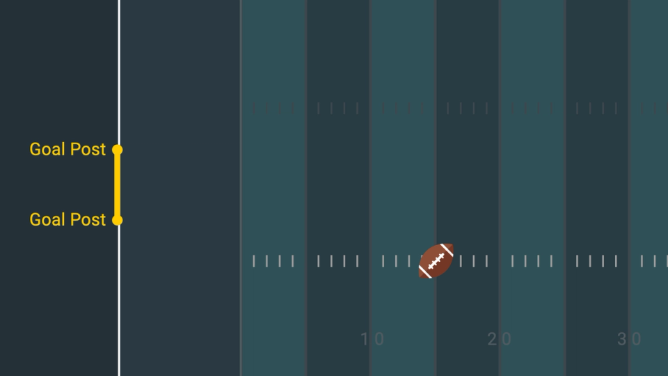
Figure 1. Sample college football field
There are two challenges to kicking a field goal. One is to kick the ball far enough, which focuses on distance. The second is to kick through the goal posts, which focuses on accuracy.
This problem only focuses on the second part: accuracy. That means our question is quite simple.
Where should we place the football on a hash mark so we have the best chance of an accurate kick through the goal posts? In other words, we are not concerned with distance, only accuracy. If we only focus on distance, then closer is better. But if our focus is on accuracy, then the problem raises interesting questions because closer is not necessarily better. This is actually a three-dimensional problem. To simplify, let’s ignore the height of the goal posts to make this a two-dimensional problem. That means we only consider length and width.
Now that we understand our sports problem, how can we formulate the concepts using math terms?
Identifying the parts
We want to maximize accuracy, but what does that mean? The answer may not be immediately obvious. Let’s pause a moment and observe some properties that may seem important.
Notice we have 3 points of interest. We have the ends of the two goal posts and we have the football. Two of these points don’t move; the goal posts are fixed. The only moving part is the football, and we’re given limitations on the football moving along the hash mark. Identifying the key parts and the moving parts is an insight in the correct direction.
Perhaps this leads us to ask how moving the football along the hash mark affects accuracy. It certainly is true as the ball moves along the hash mark that it appears more difficult to accurately kick a field goal from one position compared to another. However, the goal posts don’t move, so the distance between the goal posts remains constant. So, what determines the accuracy challenge?
Accuracy challenge
Even though the distance between the goal posts remains constant, the perception of the distance changes as the ball moves along the hash marks. We may even say that it is the angle to the goal posts that matter. We often will use a phrase like that. What does the angle mean here?
An angle requires a point and two lines. The point is the location of the football. We form the angle of interest by drawing a line from the football to each end of the posts as viewed from Figure 2. As we move the football along the hash line, our perception of how wide the goal posts are changes, as does this angle. Of course, it is only a perception as the actual width does not vary.
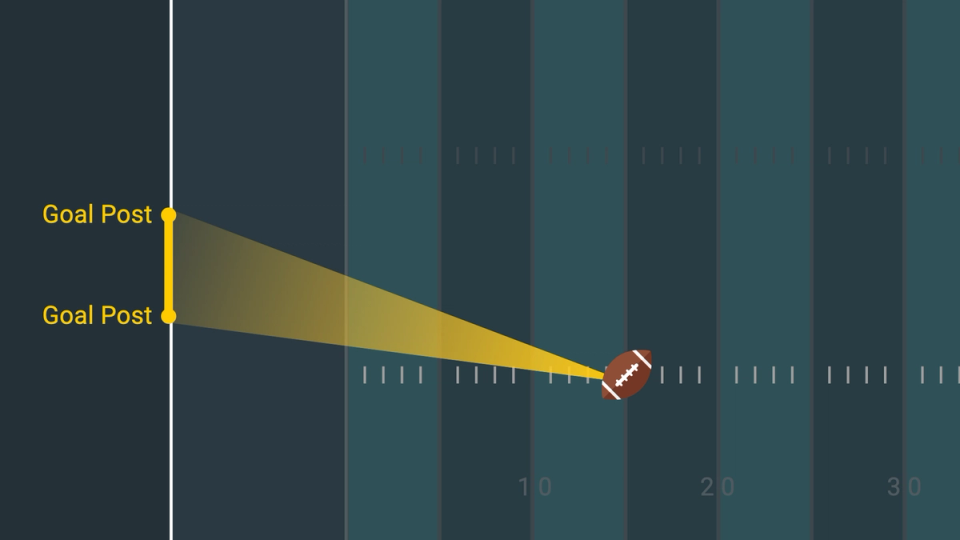
Figure 2. Creating an angle
All this made me pause and think about what really is an angle. I had studied angles before. But this time, I saw an angle as something different. I was converting a perception of identifying a better position to place the ball into something we could actually measure. This problem seemed different because I was in complete control here, but that difference made me thing about things in a new way. It made me think about what it actually meant to measure an angle. For some reason, it felt fascinating that we could actually measure an angle. If you imagine walking along the hash lines looking at the goal posts, how do you measure that angle?
A triangle appears
It helps to return to the math basics and abstract what we have. Recall we’ve identified 3 points of interest, and we’ve connected the football to both goal posts with lines. We can also connect the ends of the goal posts with a line. In Figure 2, you can see the triangle formed by connecting the goal posts. Making this connection may not be intuitive because it doesn’t change our focus, which is the angle. But the benefit in making this connection is we have now converted an angle to a triangle.
Again, a fresh perspective revealed a close connection between an angle and a triangle. Sure, I knew triangles contained angles. Here, however, my focus began with the angle and creating a triangle was more of a secondary thought. In fact, it was surprisingly simple to create a triangle from an angle by just drawing one line segment. Usually, the triangle is the main focus; the angle, or more precisely, the three angles are a component of the triangle. These subtle differences gave me a different perception of the basics of angles and triangles.
Of course, the cool thing about a triangle arriving on the scene is now I have an entire field of study, trigonometry, at my disposal. That is a huge lift because so far it felt like I was flying solo. I didn’t know IF trigonometry could be used, but I appreciated the thick textbooks with time-tested ideas at my disposal.
The logical question, even if it is a big step, is how we can use this triangle setup to maximize accuracy. Notice as I move the football along the hash lines, the triangle changes. The triangles from trig were static triangles. Perhaps the answer does not reside in the trig textbooks. Our triangle changes shape and we need to identify which triangle produces the largest angle. This dimmed my optimism about how trig was going to save my day. But let’s press forward with what we know and see where it leads.
From common sense, the larger the angle, the easier it will be to kick the ball through the goal posts. Likewise, the smaller the angle, the more difficult it will be to kick accurately. Now we know that bigger is better, at least the bigger the angle, the better. That means we can visually think about how to maximize this angle in Figure 2.
Thus, we can convert this football problem of accuracy to a math problem of maximizing an angle. Even though I created this problem over 35 years ago, I still recall the uncertainty I felt at that time. If this was a problem from a math book, or if it was on a test, I would have been quite confident that this was the correct path to a solution. But the feeling was quite different when I was creating the problem myself.
Assuming we are on the right path, let’s bring some notation and definition to the problem. First, extend the lines of the hash mark and the goal posts. These two lines are perpendicular and will intersect at a point in the back of the end zone. Define that point of intersection as O. Even though this problem clearly resides on the gridiron, we math people like to do our work on a coordinate system. So, we shift the problem from the concrete football field to our familiar abstract plane. Then, think of O as the point of origin in the -coordinate system. Part of having a math mind is the world is just one big coordinate system!
Let’s define to represent the distance in feet from the origin along the extended hash mark where we place the football. This is what we would define as the distance of the kick in a football game. The only difference is we are using feet rather than yards. In other words, a 20-yard kick means . The distance for the kick in Figure 3 is about 21 yards, or 63 feet.
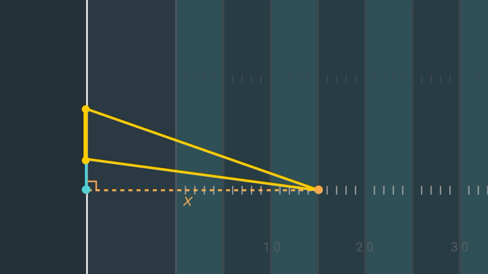
Figure 3. How our field goal angle changes as X changes
Now, let’s play with different scenarios to get comfortable with the moving parts. Start with the ball fairly far away, which means is large. I won’t use numbers yet as we are just investigating and getting a feel for the problem. Moving the ball closer, which means becomes smaller, is still better in the sense that not only does it get the ball closer to the goal posts but it improves the angle we are investigating. However, moving the ball closer only improves the angle to a point. Notice when the ball approaches the origin, the angle is small, which would make for a difficult kick as illustrated in Figure 4 where approaches 0.
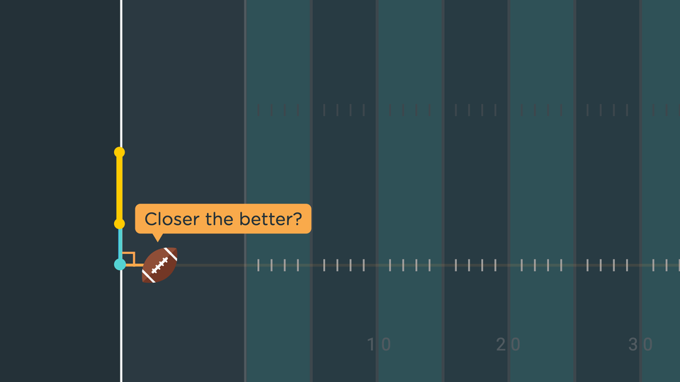
Figure 4. Closer is better to a point
Thus, as we navigate from a large value to a small value, the angle improves but, at some point, the angle gets too small because the angle becomes smaller as approaches 0. You can test this concept by viewing your television from a side angle. The width of the television represents the same thing as the width of our goal posts. For this TV analogy, the goal is to maximize the viewing angle for the TV. Start as far away possible on a line similar to the hash mark that is perpendicular to the TV and meets the wall of the TV either to its left or to its right. Then walk along this straight line to the wall. You will notice the angle to view the TV will improve for a while. However, clearly as you arrive at the wall, the angle is poor. Somewhere there must be an optimal angle, and that is the angle we are pursuing.
We have already framed our question as: what is the best place to put the ball on the hash mark to maximize our angle for kicking the field goal? We can now state our goal is to solve for such that we maximize our goal angle.
Defining “Field Goal Position”
We have defined O as the origin and the distance from O to where we place the football as . We can identify the point on the coordinate where we place the football as because point is the origin and the football lies on the -axis a distance from the origin. To simplify notation, label point simply as , which we know also represents the distance to the origin on the -axis.
Now let’s travel up the vertical, or -axis. If we define as the point of the top goal post, then the distance from this point to point O along the -axis is . Likewise, if is the point of the bottom goal post, then the distance from this point to point O along the -axis is . To remain consistent with our simplified notation, we will refer to point simply as and point simply as . Thus, in short, we have points , , and , which also represent their distances from the origin, or point O.
Now that we have our 4 points, let's connect them with line segments. Recall we already visualized a triangle from Figure 2. The points for that triangle are , , and the ball's position, . It will be handy to identify the distance between points and , so let’s define that distance as . Again, for simplicity, label the segment from point to point as segment . That means the length of one side of our triangle is . Now we can restate our goal with more precision, which is to maximize the angle opposite side , which we can label as angle as illustrated in Figure 5.
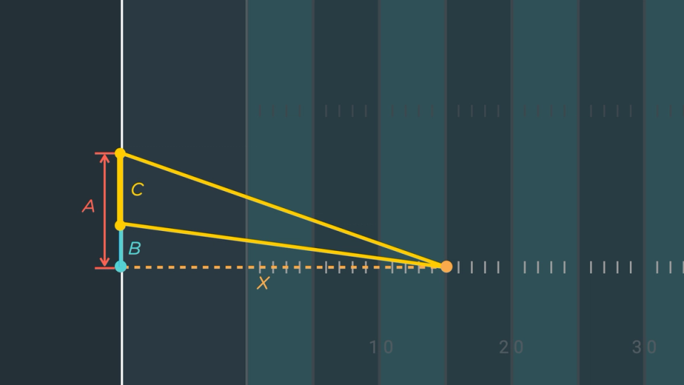
Figure 5. The field goal problem converted to math
I am using lowercase letters for angle measurements and uppercase letters for points and distances between points. So far, I have used the letters , , , and without using actual numbers. It will be more efficient to continue to use letters for a while, but let's do a quick inventory to know which letters represent numbers we know.
We are solving this problem based on the size of a college football field. The distance from the origin to point is , thus . The distance between the goal posts is feet, so . Since is , then . We don’t know angle and our goal is to solve for . It doesn’t appear we know much, but this is our setup. We will use this setup in this section and future sections, so let’s give it the name “Field Goal Position.” Before we try to solve the problem, let’s analyze angle in more detail.
Graphing our angle
We already developed a notion of what happens when we move the ball closer to the origin. This is the key hurdle to overcome. To view it from another perspective, let’s convert this notion into a graph.
Draw a graph on an -coordinate system where is on the horizontal axis and angle is on the vertical axis. If we start at , angle is . Then as increases, angle increases. We are drawing this as a smooth curve, not a disjoint or stair-step curve. This is because as you move the ball a small distance, the angle changes by a small amount. In other words, there will never be a moment where moving the ball a small distance results in a large or sudden jump in the angle. View Figure 6 to see an approximation of the function for angle and how that may be perceived as a view of the goal posts for a given value. Notice the best view appears to be between the second and third picture in Figure 6.
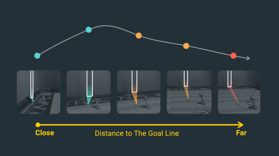
Figure 6. The angle is a curve as X changes
Recognizing that angle is a smooth curve is interesting because it reveals that hidden in this problem is a continuous function. In other words, as we move along the hash marks, the angle changes on a smooth continuous basis. That means not only does a change in position produce a change in the angle, but a small change in position produces a small change in the angle. Also, we can clearly identify a maximum in the curve at some point. This means we must find the that produces the maximum value on this curve.
Notice the irony of where we are at relative to where we started. We started with a field goal problem and it has evolved into maximizing the smooth curve we have identified. Much of Lazarus Math has been about analyzing curved lines, identifying the slopes of the curves, or evaluating the area under a curve. We converted a problem involving kicking a field goal, which had no curves in sight, into a problem that requires calculating the maximum value of a curve. Said differently, what started as a problem about straight lines and triangles is now a problem about curves. This is similar to our Buffon’s needle problem. This is why understanding how to do the math of curves is so critical: because curves are hidden in so many problems.
If you return to your TV example, can you visualize this smooth curve for the angle to view the TV as you walk closer to the wall? This is training your eye to view things from a different perspective. This is a two-part process. The first part is to stand still and think of the viewing angle of the screen as some angle measurement that has a number. The second part then is to go into motion and convert this one number into a smooth curve that we could graph. It is a wonderful skill to think about this smooth curve as you observe a change in perspective. You are seeing things very few people see. This is truly what doing math is about. Math is more about seeing than calculating. It’s about training our brain to visualize the math and finding hidden relationships and identifying properties of these hidden things. This is what math people think about when they view life. Rather than thinking about formulas, often we think of relationships.
With that moment of bliss, let’s return to the problem. Graphing a curve that we must maximize is a clever idea, but the key question is: can we identify a formula for this curve? We know the curve represents angle . How can we create a formula for angle ?
Our two problems
Before we try to write an equation, we have two problems to solve that are in our way.
First, our goal is to solve for the value of that maximizes angle . We created triangle that contains angle . It contains point , but it does not contain a side that has a length . Thus, triangle is not sufficient to solve this problem because length is an input to our function but not part of our triangle of interest.
Second, the variable that we are solving for is a distance measurement. is a distance between two points whereas angle is an angle. That leads to the interesting and difficult dilemma: how can we relate these two quantities, distance and angle measurements, which are different, like apples and oranges?
Connecting and
Let’s attack the first problem and determine if we can get to be part of a triangle that directly relates to angle . Think about how we can rewrite angle . We’ve identified triangle . But there are two more triangles whispering to us. We have triangle and . Our original triangle involves angle , but the two new triangles involve distance . How can we connect to angle ? The large triangle contains and one of the angles includes angle . Thus, let’s focus on the larger triangle. With new triangles arriving on the scene, we must usher in new definitions.
Define the angle in as angle and the angle in as angle . Notice if we combine angle and angle , we get angle . Since , , and are just measurements of an angle, we can say that angle equals angle plus angle . Then angle is angle - angle , as illustrated in Figure 7.
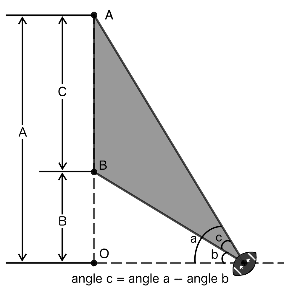
Figure 7. Solving for angle c
Pause and rotate
Let’s take a quick pause to be clear about what is legal to do with angle measurements. If I state that I make a rotation of a circle and then continue to make another , then my total rotation is the sum of the two, or . Or if I make a of a rotation in one direction, and then make a rotation in the opposite direction, then my final position is a rotation of . This illustrates that not only can we manipulate angle measurements like we manipulate numbers using addition and subtraction, but it also reminds us that an angle measurement is a measurement of rotation. Even though angle represents the angle we view the goal posts, the measurement is a rotation measurement.
We can visualize this by standing at point and facing the right goal post, then literally rotating the body while looking straight ahead to view the other goal post. The amount of the rotation is what we are measuring as an angle. We can measure it using degrees or radians or other units. Regardless of the unit, we can think of it relative to a complete rotation where we turn all the way around and finish viewing the same goal post we started with. This rotation helps clarify what we are doing abstractly with angle measurements.
Since we are already in pause mode, try to imagine how you would feel if you were solving this problem on your own, without me as your guide. Because this was a problem that I created, I initially did not know if there even was a solution that I could calculate. I still remember this feeling of uncertainty. I felt good about creating the graph of angle , which clarified the problem. But now as we get into the weeds of trying to solve the problem, it appears things are getting messy quickly.
I have taken my view of what I see from the hash mark to the goal posts and abstracted it to math terms. It seems we are quite “off road” here. Does this abstraction relate to reality? If it does, can I actually solve this math problem? We now have 3 triangles, 4 points, and 3 angles. Most of these values are unknown. Is there any hope that we can solve for all these unknowns given we only know the length of one side of our triangle?
Even though we have doubts, there is no harm in moving forward as we have plenty of paper to start again. To summarize our current status, we have the larger triangle with a base length and an angle measurement of . Thus, we have accomplished our first goal, which was to create a triangle that involves both angle and measurement .
Luck and right angles
Sometimes math is about luck, and we just found luck in our favor. What do you recognize about triangle ? Notice the segments and meet at the point . We refer to the angle at point created by these two segments as angle . Recall angle is a right angle because the extended hash mark line is perpendicular to the extended line of the goal posts. That means triangle is a right triangle. While we are counting our blessings, notice triangle is also a right triangle. If we prefer, we can refer to these two triangles as and , so we define the points of the triangle to be consistent with the points of the right angles.
More important than our notation, we should ask how this gets us closer to our goal, which is angle . Remember we can write angle as angle minus angle . That means we can now view angle as the difference between two angles of a right triangle. Truly, lady luck is on our side as illustrated in Figure 8.
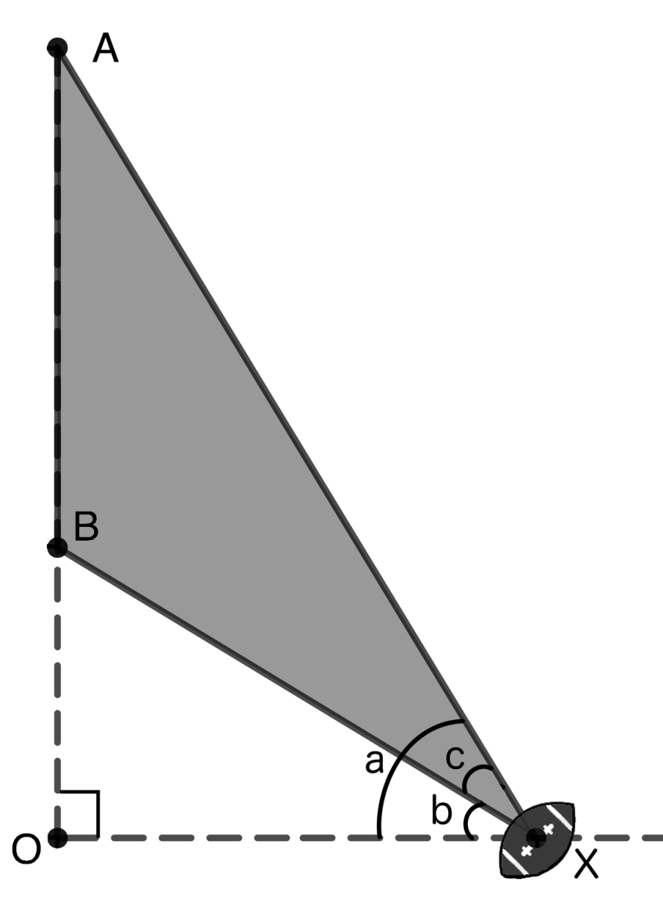
Figure 8. Two right triangles
Adult math: connecting an angle to a distance
Now, our second problem is creating an equation where we combine an angle measurement with a distance measurement. Remember when we were working with a unit circle and we used the sine and cosine functions? Then, when we worked with the Madhava-Leibniz series, we used the tangent and inverse tangent functions. We categorize these functions as trigonometric functions. Notice these magnificent functions perform the magic of connecting angle measurements to distance measurements.
I specifically remember an “aha moment” when I worked on this problem. By college, I had been using the sine and cosine functions for several years, so I was quite familiar with them. But I never appreciated the magic they performed until I was working on this field goal problem. Up until that time, when I used the sine and cosine functions, it was very prescribed because they were given as part of textbook problems. However, for this field goal problem, I was not even thinking about these functions. There was not a textbook to suggest using these functions. There is a big difference between being told to use these functions and identifying that these functions can be used without any hint they are needed.
It’s like when you are a kid, you do things because your parents tell you to. When you become independent and make your own decisions, sometimes you stumble back into doing something you did routinely as a kid, but now you are doing it because you see the big picture. I remember thinking that at this moment, I had become an “adult” with math. Math was not something I did simply to respond to an external request. Now I’m taking ownership of my math and considering the big picture. I viewed these functions, and all of math actually, as available tools for me to use whenever I wanted. This is quite different from viewing math as a subject for me to study.
It is difficult to put into words what a turning point this was in my life, even though it was such a small step in math. It changed from “math acting on me” to “I’m acting on math.” Until you reach that point, math is difficult and feels heavy. After that point, math is still difficult, but it doesn’t feel as heavy. It doesn’t mean you will solve problems any faster, but it is now from a different perspective. This is similar to being an adult and making decisions not because someone tells you to, but because you choose to.
Putting our trig to the test
With that “aha moment” aside, let’s test our trig function muscle to see what it can do. How can we use these trig functions? We mentioned lady luck was on our side when we identified right angles and right triangles. This is because we can use a trig function to convert an angle measurement to a ratio of side measurements. Think about how wonderful that is. We just imagined an angle as a rotation. Now, we’re saying we can measure that rotation by converting an angle to a triangle and then doing some math magic with the length of the sides to measure the angle.
Let’s remind ourselves of the moment when we imagined standing on the hash mark at point facing one post and then rotating to face another post. We did this to get a feel of an angle measurement. Now, imagine that we can measure distances in our triangle and then do some math magic to calculate the measurement of that rotation. Doesn’t this seem a bit bizarre?
To me, the part that seems fascinating is if I just focus on the rotation, then the ends of the goal posts appear as rather random points of my vision. Think of it this way: Start by facing point , the right goal post. Then rotate left until you face the left goal post, or point . This rotation is our angle . However, I could have chosen other points that were part of the same rotation. I just happened to choose the obvious points, and , which are the goal posts.
For example, two other points I could have chosen are the points halfway between and and halfway between and . I should still arrive at the same angle measurement by choosing these two points. What we’re stumbling on here is the notion of similar triangles. Similar triangles are triangles with the same angles, and thus the same shape, but different sizes. I did not use the notion of similar triangles when I solved for angle , but I did use the notion later in the story.
Returning to the task at hand for solving for , which trig function should we use? We’re free to choose any; remember we are now “math adults.” The two most commonly used are the sine and cosine. However, both involve the hypotenuse and we don’t have any known measurements on the hypotenuse for either triangle. Remember a third function is the tangent function, which is opposite / adjacent. Specifically, Figure 9 illustrates the tangent of angle is and the tangent of angle is . Since we know and , and the variable of interest is , the tangent seems to be a good choice. The tangent of angle and the tangent of angle is .
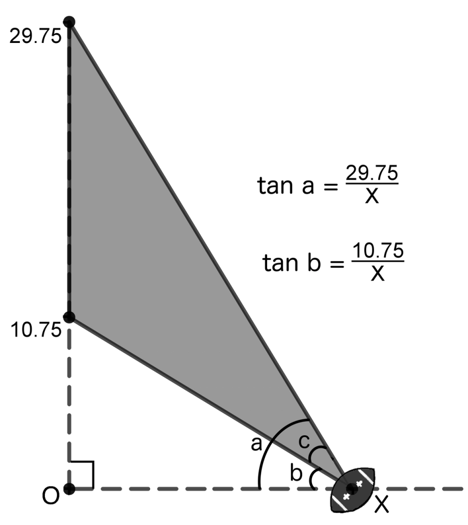
Figure 9. Connecting an angle to a distance
Here we are at another fork in the road. We know that angle is angle minus angle . Now that we’ve introduced the tangent function, we have embedded and into a function but not . We know because all 3 are angle measurements. When we applied the tangent function to these angle measurements, we gained the ability to connect to a distance measurement, but we lost something in the process. What we lost is the additive relationship between these three numbers. We cannot say that tangent equals tangent plus tangent . Nor can we say that tangent minus tangent equals tangent .
Some functions preserve addition when applied and some don’t. For example, we could multiply and by 2 and still preserve the relationship. However, if we square each term, or apply the square function to each term, then we lose that relationship.
So, after tremendous progress, it appears we’re stuck again. I remember how I felt stuck at this point. It appears there is no way to connect to . Can we restore this connection? If so, how? We have two equations that connect and to distance , but neither involves angle .
Undoing the tangent function
It seems like if we could somehow “undo” the tangent function, then we return to the original numbers and we can restore our connection. Is this possible? When we discussed the Madhava-Leibniz series, we introduced the inverse tangent function. Remember the inverse tangent function is exactly what it sounds; it can “undo” the tangent function. This is similar to a hammer that has a “do” feature (a head) that pounds nails and an “undo” feature (the claw) that removes nails. That means we can take the inverse tangent of the tangent of angle and we are left with angle . What fantastic functions we have in inverse trig functions!
We have an equation, so to preserve equality, we take the inverse tangent of both sides. This may seem like an odd thing to do to manipulate an equation, especially if you are not familiar with the inverse tangent function. You can think of it as taking the inverse tangent of equal expressions will produce equal expressions after applying the inverse tangent. We can do this to both angle and angle .
Because I felt truly stuck after losing the connection to from the tangent function, this was another “aha moment” that I still vividly remember. Up to this point, I always viewed functions like the inverse tangent as another function I must learn, another function that made things seemingly unnecessarily complicated. However, while working on this problem, I gained a great appreciation for what the inverse tangent function does, even a sense of awe that it actually works. It is another example of a real-life problem for which there doesn't seem to be a solution at first. You actually feel the weight of being stuck. Then, almost out of nowhere, you remember this tool you learned and, for the first time, it seems useful, and useful in a surprising and satisfying way. Another “adult moment!”
Let’s apply this undoing process to restore and . Here are our new equations.
Now, restore and by converting the “doing” and “undoing” as doing “nothing.” While we’re at it, let’s substitute our distance measurements.
Since and are completely free from the tangent function and their values did not change in the process, we can write . Now, equals the difference between the two inverse tangent expressions.
Equation found and how to solve it
Wow, that was a lot of work. Through the weeds, let’s recall why we went through this process. Remember represents the angle measurement we’re trying to maximize. This angle changes based on the value we choose for . Now we have an expression for angle that is a function of . Even though this is a messy expression, it’s quite remarkable we can make this connection. Remember, we not only had to connect a distance measurement to an angle measurement, but that distance was not directly connected to the angle. It was indirectly related, which is why we created 2 different triangles.
To get a feel for how remarkable it is that there is this connection, return to our TV example. This example is the same concept as our football example, which means we have similar triangles but with different values. That means we can use the same setup and calculate a different and but reuse the same equation. That means you can stand some distance from your wall and use this same equation to solve for the angle of viewing your TV. Then, you can take a step closer to the wall, remeasure , and recalculate the new angle. Isn’t it special that we can convert that distance to an angle measurement that does not even touch the ending point of , which is the point on the wall you are measuring to? Intuition would indicate that to measure the angle, we would need to measure the distance to the TV, but we don’t.
That means we’ve created an equation, or even more specifically, a function. This allows us to feed any input value we want that is a positive real number, and the result will be some value which represents the angle we create when our distance is from the wall.
This is not the only thing I find fascinating. Think about how we converted a difficult measurement into an easy measurement. Measuring angle exactly would be extremely difficult to do. Perhaps we could get a rough approximation by using a protractor and some setup. Even with all that work, how accurate would it be? Here, we simply measure and , which are easy distance measurements we can get with a tape measure with decent accuracy and ease. These values do not change. So the only other measurement needed is , which is another simple tape measurement that is easy and quite precise relative to an angle measurement.
Even though we likely do not need a precise angle measurement, the simple fact that we can calculate it easily and accurately is satisfying. Certainly, our solution feels near, so let’s “get to the end zone.”
We sketched a graph of angle in Figure 6, so let’s reapply that important perspective by repeating it in Figure 10. We now know the formula for this graph. This means we are proposing that the difference between two inverse tangent functions is the formula for angle . Who would have thought that?
Figure 10. Review of our angle c graph
I know I certainly did not. Even though it feels like we are near the end because we have the equation for , I remember my thoughts and feelings were anything but confident. In fact, I remember this was another crossroad for me because I seriously doubted I was on the right track. Again, because this was my own idea and I was so far from my starting point, my instincts told me it was highly unlikely this was the solution to the field goal problem. Can you imagine doing this problem on your own without any outside help and arriving at a “bizarre” equation for angle which takes the difference between two inverse tangent functions. How confident would you be that you were on the right path and this is actually the solution to the field goal problem?
But, like a good pilot, you must trust your controls more than your instincts. I felt that everything I did was sound. Even though this equation does not appear remotely connected to my field goal problem, let’s ignore the doubts and move forward.
Maximizing
Now everything is in place to calculate the angle based on distance because we have a formula for . But how do we maximize ? In other words, how do we choose the specific value for that produces this maximum angle ? We could use a trial-and-error method by selecting different values and calculating angle using the formula. But that would be time consuming (OK, when did we start worrying about time?!) and we likely would only arrive at an approximate answer. Now is when we put our foot down and issue a demand. Our demand is we only want to do this once and we want the answer to be exact. No 2, 3, or 4 rounds of guessing and no approximation. Once and exact. That is our request. Is there math magic that can achieve our demand?
A summary of our demand is we want the that maximizes the difference of two inverse tangent functions. Maximizing is different from solving. Solving is more of an algebra problem. Solving means given any input , calculate . Maximizing is given the maximum value for , whatever that maximum value is, then identify the input value that produces this maximum value. Doing this maximizing work with the difference of two inverse tangent function seems monumental.
As we have learned many times, what appears impossible with algebra is possible with calculus. Recall one of the gifts of calculus is we can start with one equation and then create another equation, called the derivative equation, that represents the slope of the original equation at any point. If you review our function in Figure 10 and consider a tangent line at the maximum point, the slope of that tangent line is 0 because the line is horizontal and parallel to the -axis. That means if we can determine the derivative equation, then we can set that equation to 0. The solution for that equation is the we need to maximize our function and thus maximize our angle. This may seem like a giant leap, but it is one performed countless times in calculus and quickly becomes routine. If this is your first time using a derivative to identify a maximum of a function, it will seem foreign. But, like riding a bike, it quickly becomes natural.
Let’s return to calculus and identify our derivative equation.
Calculating a derivative
The neat thing about this derivative equation that we are looking for is that it only needs to be solved once. For example, the derivative equation for the sine function is the negative cosine function. It truly becomes a formula that we can use and reuse to our mind’s content. So is there a derivative equation for the inverse tangent function?
The answer is yes. This derivative equation is actually something we have already encountered. Recall in our Leibniz problem, we had a messy area problem that simplified to the area under the curve and above the -axis. We needed to find a function whose area function is . The solution was the inverse tangent function.
It just so happens that when we want to create a function for the slope of a curve, we actually perform the reverse operation that we do with our area function. In other words, just like addition and subtraction are opposite operations, so is identifying a slope of a curve and finding a function given its area. This is an amazing thing that we are going to gloss over here. We’re going to jump to the conclusion that the derivative equation for the inverse tangent of is .
This is the main part for our solution, but we have two details to unravel before we are in the end zone.
More calculus magic
First, we do not have the inverse tangent of , but we have the inverse tangent of . If it was just the inverse tangent of times , that would be easy as that would create the function . In other words, the multiplicative factor 29.25 is just passed through. It is slightly more complicated if we are dividing by . Since we are dividing by , the derivative equation changes to . Notice the changes: (1) the fraction is now negative and (2) the first term of the denominator is rather than 1. We’re going to skip over the reason why this is true and just focus on the result.
Our second issue is we have two terms that include the inverse tangent function. Notice we subtract the second term from the first. This second issue is easier to solve. The solution is to apply the calculus magic to both terms separately, then take the difference between the results. You can think of it as preserving the operation of subtraction through our calculus magic.
Let’s perform the same magic on the second term. Since the second term is similar to the first, we’ll replace 29.25 with 10.75, then subtract the second term from the first.
\text{Original expression: }tan^{-1}(29.25/X)-tan^{-1}(10.75/X)
Notice we are subtracting the second term from the first term and the second term is negative. Subtracting a negative term is the same as adding a positive term:
This slope expression represents the slope of our field goal angle at any value . We’re quickly going through the math, but let’s take a quick pause to understand what this slope expression represents. This is the slope expression for the graph of angle in Figure 10. Thus, if we input a value, say 5, which represents 5 feet from the end zone, then the result will produce a slope for angle . How can we interpret that result?
Interpreting a slope
You can think of it as how fast that angle is changing for a small change in . Here the sign is important as well. If we go left to right on the graph, we see a fairly large increase in the graph at first. That translates to a fairly large positive number. Eventually, the graph decreases which means the slope becomes negative. Our goal is to identify the exact point it goes from going up, or positive slope, to going down, or negative slope. That exact point is when the slope is 0.
Let’s summarize our work in 3 important formulas.
- Formula to calculate angle : tan^{-1}(29.25/X)-tan^{-1}(10.75/X)
- Slope (derivative) expression for angle :
- Setting the slope expression to 0:
Solving for … finally
Now, we are truly at the point where we can use algebra to solve for . Performing the algebra to solve for is like a teenager's bedroom—our clean math gets dirty with little effort. We need a common denominator, which creates this mess.
Despite the mess, lady luck reappears because the right side of our equation is 0. That means the left side must be 0, and the only way the left side is 0 is if the numerator is 0 (and the denominator is not 0). Thus, let’s dismiss the denominator and set the numerator equal to 0. While we’re rewriting, we might as well combine factors.
The end is near! All that remains are terms and constants, so combine each.
The solution is . Distance must be positive, so the initial solution is .
Return to football and making sense of it all
Wow, we actually solved for ! Let’s recall what represents. From our definition of “Field Goal Position,” is the distance (in feet) from the back of the end zone to kick our field goal. Thus, the optimal distance to kick the field goal is 17.73 feet from the back of the end zone.
The end zone is 10 yards long, which is 30 feet. That means the optimal spot to kick is less than 30 feet which means it is in the end zone. I admit, this is a shorter distance than I anticipated. Because I thought I could easily have made a mistake somewhere, I performed a couple of sample tests. First, I calculated angle when .
which is about 27.5485 degrees. We all have a feel for a 45 degree angle. Half of 45 is 22.5, so just a little more than half a 45 degree angle is the best we can hope for.
To confirm we have a maximum angle, let’s calculate the angles for distances slightly shorter and longer to the back of the end zone.
For slightly longer, let , then . For slightly shorter, let , then . Notice the largest angle measure among the 3 values of corresponds to . This gives us confidence that we identified the maximum angle .
Of course, if we wanted complete confidence we solved this problem correctly, we could graph angle based on our formula. Here is the graph for angle in radians. For comparison, I thought it would be interesting to also graph the angle for the field goal if the ball was placed in the optimal position. The optimal position is in the middle of the field and not on the hash marks. It should be common sense that if the ball is between the goal posts, then closer is always better and farther is always worse.
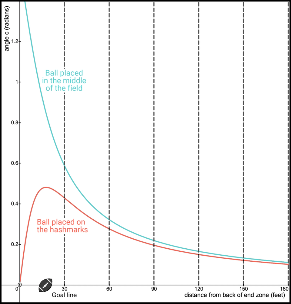
Figure 11. Compare best-case and worst-case angles
To be consistent, I am still measuring in feet, so divide everything by 3 to convert to yards. Thus, the 30-foot interval is a 10-yard interval. Also, there are 30 feet, or 10 yards, from the goal line to the back of the end zone. The final measurement on the right, 180 feet, is midfield, which is a kick of 60 yards or 180 feet, which is also 50 yards from the front of the end zone. Notice there is not much difference in the angle from this distance regardless of whether you place the ball in the best position, in the middle of the field, or the worst position, on a hash mark. If you stood at the 50-yard line on a football field, the angle between the posts will appear about the same regardless of whether you are in the middle of the field or on a hash mark.