Connecting to something of interest

“Compound interest is the eighth wonder of the world. He who understands it, earns it; he who doesn’t, pays for it.” - Albert Einstein

Equivalent

We’ve been dancing with hall-of-fame-type math so far. In my career as an actuary, I’ve encountered interesting math, and here is an example I can’t resist sharing. It is one that connects the finite to the infinite.

This math is connected to finance and is related to a previous story where we doubled our investment. Remember in that example, we started with interest so that $1 grew to $2 after one year. We get that result simply by using the formula $$1 × (1+i)$ where $i$ is our interest rate.

The job of an interest rate is to measure the rate at which money changes. There are several ways to measure the rate of change, meaning there are several types of interest rates. You are likely familiar with the concept of compound interest. This is where interest earns more interest. For our “double in one year” example, we had the good fortune to have the compound interest rate equal to 100%. Let’s scale back a bit and let our compound interest rate equal 10%, still a hefty rate but not crazy good like doubling in one year.

If our compound interest rate $i$ is 10% and we invest $100 for one year, then after one year, our fund increases to $100 \times (1+10\%)=110$. In the actuarial world, we reserve a special word “equivalent” to represent a key concept. We would say that $100 today is “equivalent” to $110 in one year if our compound interest rate is 10% per year. Notice the word “equivalent” is not the same as “equals.” We’re not saying $100=110$. We use the word equivalent because if our interest rate is 10%, prudent investors would be equally satisfied with $100 today as they would be with $110 in one year, ignoring all other factors of finance (like whether they need the money more today or in one year). Here is a graph of how this fund grows over time.

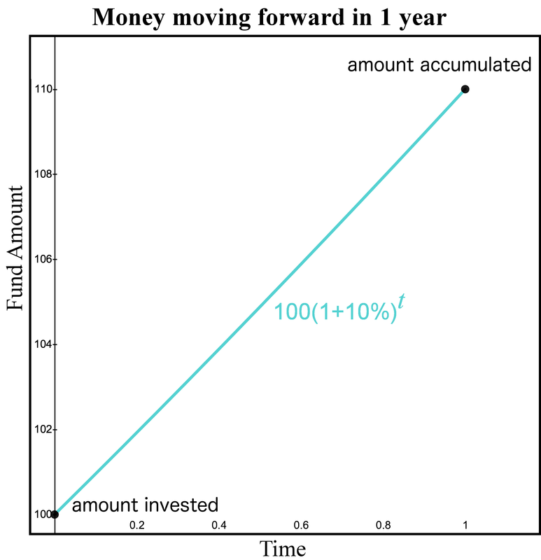
The horizontal axis represents the amount of time since the initial deposit occurred. The vertical axis illustrates how the fund increases over time from compound interest. This graph may appear to be a straight line because we are only viewing the first year of the investment. However, if we view the investment over a longer period of time, such as 20 years, we can see how the slope of the fund increases over time.

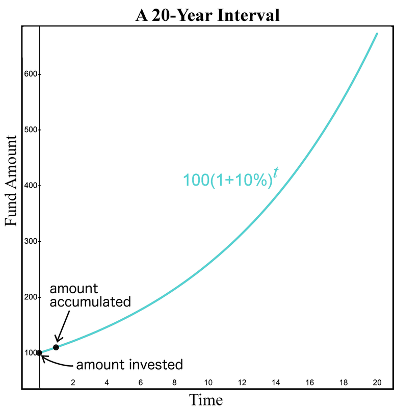
The increase in the amount of the fund changes over time because of compound interest. We normally view this graph left to right which means we observe how interest moves money as time moves forward.

Moving money backwards

Notice we can travel backwards in time and ask the question: If I have $110 in 1 year, what is the equivalent amount of money I would have today if the interest rate is 10%? Observe we already have our equation. This time our unknown is our initial investment. Since we know the ending value is 110, simply divide both sides by $1+10$%. Then, our new equation is

$$\text{Today’s value} =\dfrac{ \text{Value in one year}}{1+10\%}=\dfrac{110}{1.10}=100$$

This reproduces our initial fund. We can graph this relationship similar to how we graphed the fund increasing as time increases. The horizontal axis remains time. But now let the horizontal axis represent the amount of time we go back into the past. Since we are starting with a fund value of 110, we set that as the fund value at time 0. Then, as we increase time, we are increasing how far BACK in time we are going. Thus, we observe how the fund decreases as we move backward in time.

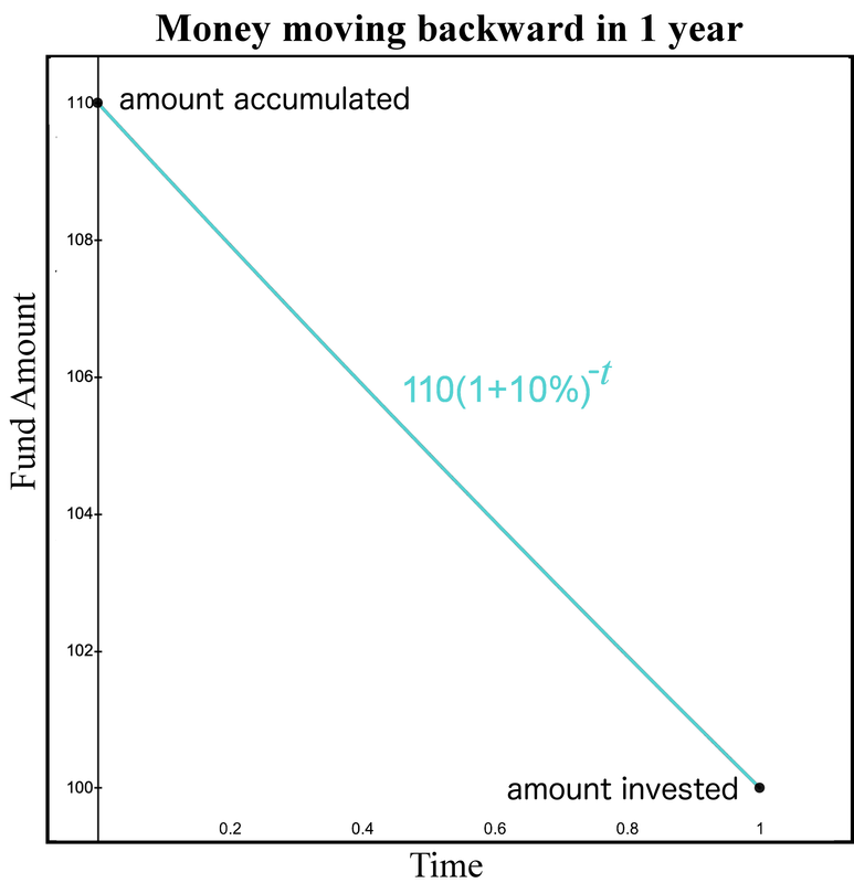
Our main takeaway here is we have a method to “move money forward” one year by multiplying by $(1+i)$. This produces a value in one year that is equivalent to the starting value. Likewise, we can reverse the process and “move money backward” one year by dividing by $(1+i)$. If you prefer, you can move money backward one year by multiplying by $(1+i)^{-1}$. Notice the -1 exponent represents going backward in time 1 year.

Good. We can think of the $110 in one year as two parts. One part represents the original investment, called the principal, which is $100. The second part is the interest earned, which is $10.

Focus on the interest

For now, let’s ignore the principal part and focus on the interest part. In our example, the interest is earned in one year and the amount of interest is $10. Thus, think of the $10 interest payment as a cash flow that occurs at time 1. What if we wanted to know the value of the time 1 interest cash flow at a different time, say at time 0? In other words, what is the equivalent value of the interest at time 0? We already identified that a cash flow of $100 at time 0 is equivalent to a cash flow of $110 at time 1. How do we calculate the value at time 0 interest cash flow which is worth $10 at time 1?

This may appear to be an odd question. But just think of it as a math question and ignore the business context for a moment. We have a time 1 cash flow of $10 and we want to identify the equivalent value of this cash flow at time 0. Notice this requires using our "move money backward” method. Given our time 1 value is $10, we can calculate today’s value by dividing by the factor 1.10. Thus, based on a 10% interest rate, the $10 at time 1 has a value today of $10 \times 1.10^{-1} = 9.09$.

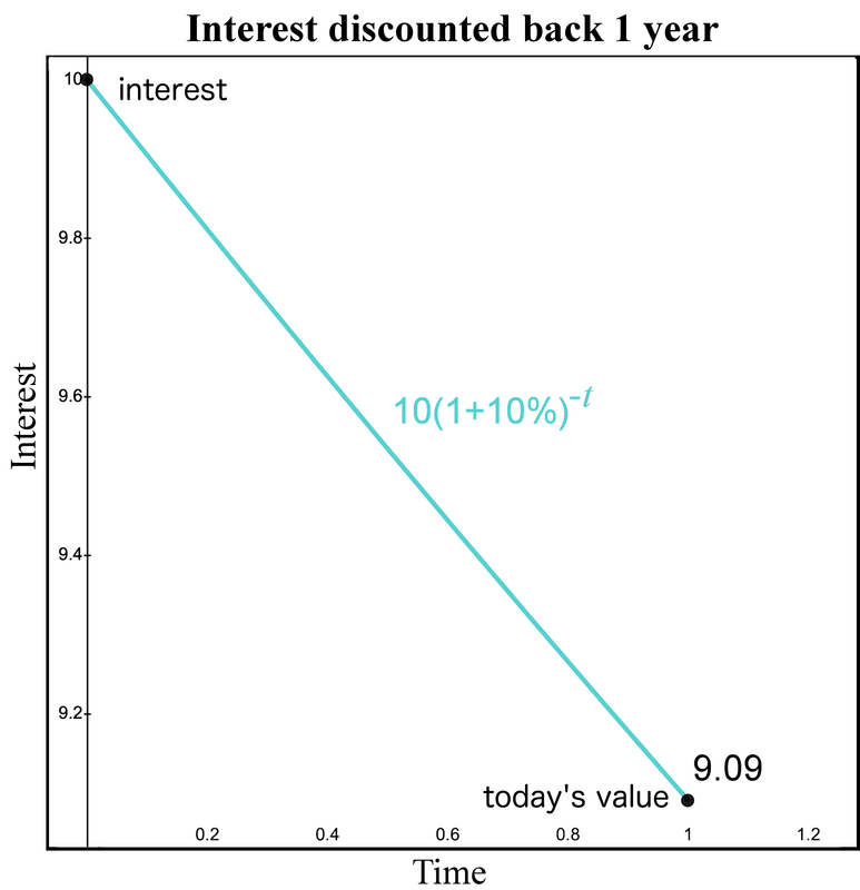
If this is still confusing, notice how similar this graph is to the previous graph. The only difference is the first graph started with $110 and the second graph started with $10. But both moved backward in time the same way by dividing by 1.10. This means a time 0 cash flow of 9.09 is equivalent to a time 1 cash flow of $10 using a 10% compound interest rate. Now that we performed the math, let’s understand the business context.

What does this 9.09 represent? Return to our initial story where you invested $100 in the bank and the bank promised to return your $100 principal payment in 1 year and to pay you $10 in interest. Note that this is not the only way the bank could pay you interest.

Equally satisfied

Another option is you still agree to invest $100 in the bank for 1 year. That means you deposit $100 in the bank at time 0. The bank still promises to return your $100 principal in one year. Also, the bank still promises to pay you interest on the investment at a 10% rate. If the bank pays you the interest at the end of the year, then the amount of interest the bank pays you is $10. But the bank could decide to pay you interest at time 0 rather than time 1. There is no rule that states the interest payment must occur at time 1. It can occur at any time. However, our goal is that the amount paid is always equivalent to $10 at time 1. Thus, if they pay you interest at time 0, the amount of interest they must pay is $9.09 because that is equivalent to paying you $10 at time 1. Notice we now have two ways to pay interest that are equivalent. You and the banker should be “equally satisfied” with either arrangement. Let’s refer to this bank that pays interest at the beginning of the year as Bank 1.

Why would you be “equally satisfied” with this arrangement? You would be “equally satisfied” because you could take the 9.09 time 0 interest that Bank 1 paid you and invest it for one year at 10% at another bank, call it Bank 2, that pays interest at the end of the year. Then, we identify the value in one year by using the “move money forward” strategy and multiply by 1.10. Thus, the 9.09 deposit at time 0 at Bank 2 increases to $9.09 × 1.10 = 10.00$ at time 1. This means you still finish with $100+10$, or 110, which is the same amount you finish with if you earn interest at the end of year. Here is a table that documents our cash flows.

Time	Activity	Cashflow
0	You deposit $100 at Bank 1	-100
0	Bank 1 pays you interest at the beginning of the year	+9.09
0	You deposit $9.09 at Bank 2	-9.09
1	Bank 1 repays you your $100 principal	+100
1	Bank 2 pays you principal and interest on your 9.09 deposit	+10

In summary, your total cash flow at time 0 is -100 and your total cash flow at time 1 is +110, which is why you are equally satisfied if Bank 1 would have paid you the interest at the beginning or at the end of the year.

So far, we’ve introduced two different ways to pay interest. We have used the phrase “equally satisfied” to connect these two stories. We’re now going to give a technical term to clarify how these two stories connect. The key is to understand that our measurement of interest is measuring the same thing but from two different perspectives. A different example will clarify this. We can measure 36 inches as either 3 feet or 1 yard or 36 inches. If you don’t understand each of these units, it would be difficult to identify we are measuring the same distance, just using different units of measurement. We’re doing the same thing here where we analyze a set of cash flows using two different measuring techniques. We will calculate a different numeric result for each method, but that is because they have different definitions. However, they are only two different perspectives of the same thing, just like 3 feet and 1 yard are two different perspectives of 36 inches.

With that thought in mind, remember our “equally satisfied” story is all based on our 10% interest rate. Notice we started at time 0 with a $100 investment that earned interest of $10 at time 1. Then, we moved that money back to time 0 by dividing by 1.10 to get 9.09. What is the rate of interest you earned if you are paid $9.09 at time 0? The initial investment is $100 and the amount of interest is 9.09. Thus, the rate of interest is $\frac{9.09}{100}$, or 9.09%. But we started our story with a rate of interest at 10% and we always followed our “equally satisfied” method of moving money forward and backward using the 10% interest rate. How do we reconcile our different interest rates? We reconcile by giving different definitions to the interest rates (think feet and yards).

Notice we calculate the 10% interest rate as $\frac{10}{100}$ when we pay the interest of $10 at time 1, and we calculate the 9.09% interest rate as $\frac{9.09}{100}$ when we pay the interest of $9.09 at time 0. We can say the interest paid at time 1 is interest paid “at the end,” and the interest paid at time 0 is interest paid “at the beginning.” We give fancy names to both of these concepts. When it is paid “at the end,” we say interest is paid “in arrears.” When it is paid “at the beginning,” we say interest is paid “in advance.” Thus, the interest rate paid in arrears is 10% and the interest rate paid in advance is 9.09%. Because we used our “equally satisfied” principle for moving money forward and backward, we can say that a 9.09% interest rate in advance is equivalent to a 10% interest rate in arrears. Again, we carefully choose the word equivalent. In short, a 9.09% interest rate in advance and a 10% interest rate in arrears are just different perspectives of the same thing.

Let’s review the math we have used so far. But, to make it easier, let’s use some common notation. We usually let $i$ represent the interest rate in arrears and $d$ represent the interest rate in advance.

Interest paid in arrears (at time 1) = 100 x (1 = $i$) - 100 = 100 x $i$

Interest paid in advance (at time 0) = $\frac{100i}{1+i}$

Notice if we change the initial investment from $100 to $1, the result simplifies to:

Interest paid in arrears (at time 1) = 1 x (1 + $i$) - 1 = $i$

Interest paid in advance (at time 0) = $\frac{i}{1+i}$

Since we let $d$ represent the interest rate paid in advance, we arrive at the important conclusion that $d=\frac{i}{1+i}$. Recognize this is our key conversion formula, just like 3 feet equal 1 yard is the way to convert feet to yards.

Connecting interest rates

This is a key takeaway, but we don’t have to stop here. Let’s play with this by simplifying and removing the fraction.

Multiply both sides by (1 + $i$): $d$(1 + $i$) = $i$

Distribute within the parentheses: $d+id=i$

This tells us that the product of interest in advance and interest in arrears equals the difference between the two. It is an interesting formula (no pun intended) where we connect two terms using multiplication on one side and subtraction on the other side. Here's another version of this formula.

Discounting with interest

Notice we have two expressions for $d$. The first was $\frac{i}{(1+i)}.$ We think of the process of dividing by $(1+i)$ as a way of moving money back one year. Remember, we moved back the $110 one year by dividing by $(1+i)$ and we moved back the $10 interest by dividing by the same $(1+i)$. We call the process of dividing by $(1+i)$ “discounting with interest.” Notice if we review our two expressions for $d$, we can see that we can go from $d$ to $i$ in two ways. One way is dividing by $(1+i)$. The second way is by multiplying by $(1-d)$. Since multiplying by $(1-d)$ is doing the same thing as dividing by $(1+i)$, then we can also say that multiplying by $(1-d)$ is also “discounting with interest.”

Recall we started by multiplying by the factor $(1+i)$ to accumulate money forward. Thus, we’ve identified that if we want to accumulate money forward, we multiply by $(1+i)$, and if we want to move money backward, we divide by $(1+i)$ or multiply by $(1-d)$. Using the same logic, we can accumulate money forward by dividing by $(1-d)$.

Moving money

Here’s a table that summarizes our findings so far.

Move money	Interest paid in arrears ($i$)	Interest paid in advance ($d$)
Forward	Multiply by (1 + $i$)	Divide by (1 - $d$)
Backward	Divide by (1 + $i$)	Multiply by (1 - $d$)

Since the factor (1 - $d$) moves money backward, it makes sense that it also moves an “interest rate backward.” Hence, if we start with interest in arrears, $i$, and we pay it in advance, we move it backward by multiplying it by (1 - $d$). The result is we converted interest in arrears to interest in advance. Hence, $i$(1 - $d$) = $d$, which we identified earlier, but now we have a way to interpret this result.

In summary, if we have an interest rate in arrears and we want to convert to an interest rate in advance, we can either divide by (1 + $i$) or multiply by (1 - $d$). Likewise, if we have the interest rate in advance and we want to calculate the interest rate in arrears, we either multiply by (1 + $i$) or divide by (1 - $d$). Again, if it seems odd to manipulate interest rates forward and backward in time, you can assume the investment is $1, which generates actual cash flows.

Here is a table of 3 sets of cash flows that are equivalent based on interest rate $i$ paid in arrears and interest rate $d$ paid in advance. Because these cash flows are equivalent, we should be “equally satisfied” with each.

Equivalent cash flows	time 0	time 1
An initial deposit	1
Interest paid in arrears		$(1+i)$
Interest paid in advance, principal repaid	$d$	1

In search of the infinite

Notice we have defined two different interest rates: one that pays interest at the beginning of the period and one that pays interest at the end of the period. If the period we are measuring is a timeline, then these rates serve as "bookends.” But our goal in this section is to connect things that are finite to the infinite. These bookends represent the finite. Is there an interest rate that connects to the infinite?

Let’s summarize our two bookend options. One pays all the interest at the beginning of the period, which we call interest in advance, and we use $d$ to represent this rate. The second pays all the interest at the end of the period, which we call interest in arrears, and we use $i$ to represent this rate.

Here is a third option. It pays interest on a continual basis for the entire year. It may be difficult to imagine paying interest on a continual basis. I like to think of it as being paid in very small increments, such as 0.0001 part of a year. However, if you want a continuous analogy, you can think of being paid interest in the form of liquid gold being poured into your account at every moment. Given this scenario, how much interest, or liquid gold, are you paid?

The amount of liquid gold you are paid is a constant rate based on how much money is in your fund. In our example, we started with $100. However, the trick here is that when you receive interest in the first moment, it is reinvested. Remember when we identified the interest in advance was equivalent to the interest paid in arrears, we took the 9.09 interest paid in advance and we reinvested it to the end of the period. When we use the continuous rate, the amount of liquid gold being poured at any moment is slightly more than the amount of liquid gold that was poured the previous moment because the liquid gold poured the previous moment has become principal and earns interest. This clearly gives us an infinite process, which fits our goal.

Constant rate of change

We’ve created a process where we are earning and reinvesting interest at a constant rate. We want to calculate that constant rate. Before we calculate, first, let’s get a sense of what this constant rate may be. How does a continuous compound interest compare to one that pays in advance or one that pays in arrears? Remember the interest paid in advance and the interest paid in arrears are our bookends. Thus, it seems logical to think that interest that is paid on a continuous basis is an average of the two. If we assume the interest paid in advance is 9.09%, then we know the equivalent interest paid in arrears is 10%. What is the interest rate that is equivalent to these rates but is paid on a continuous basis?

How do we calculate this constant rate of interest that is being paid? Notice we have a continuous compounding process at play. Also, notice we need a method to “move money forward” similar to what we did before when we multiplied by 1 + $i$.

There is a good chance you are not an actuary, so the theory of interest may not excite you like it does me. But our goal is for math to come alive, and this is where this seemingly calm story about interest rates can illustrate a wonderful principle in math.

Notice our goal is to find a continuous rate of interest that accumulates money at the same rate as $(1+0.10)^t$. Since our variable, $t$, is an exponent and the base, $1+0.10=1.10$, is a constant, this is an exponential function. We have discussed exponential functions before in Lazarus Math. There are many interesting nuggets buried in an exponential function that it takes many stories and perspectives to appreciate them.

Recall we identified that the pitch of a note doubles every octave. The fundamental frequency is 440 for A4, 880 for A5, and 1,760 for A6. This is an exponential process because change is occurring by multiplication. We naturally think that change occurs more in a linear fashion. Today has 24 hours and tomorrow has 24 hours. The total number of hours we have today and tomorrow is $24+24=48$. We are also familiar with the principles of the graph of a line.

How many exponential curves are there?

If we have two points in the $xy$-coordinate system, we know there is one and only one line that can connect those two points. We have two points in the $xy$-coordinate system we are considering. The time 0 fund value is 100 and the time 1 fund value is 110. Thus, the two points are $(0, 100)$ and $(1, 110)$. We know there is one and only one line, or linear function, that connects these two points. The equation for that line is $y=100 \times (1+0.10t)$.

How many exponential functions connect $(0, 100)$ and $(1, 110)$? We know $y=100 \times (1+0.10)^t$ is one such exponential function. Is that the only one? The intuitive answer from our story so far is there must be more than one exponential function because we also identified a different way to connect these two dots by using the interest rate in arrears $d$. That means another way we can connect these two dots is by using the equation $y=100 \times (1-0.0909)^{-t}$.

But is this really a different exponential curve? Not only does the function using $d=0.0909$ connect the same two points $(0, 100)$ and $(1, 110)$ as the equation using $i=0.10$, but they are identical functions for any input $t$. For example, if $t=2$, we can write $y=100 \times (1+i)^{2}=121=100 \times (1-d)^{-2}$, where $i=0.10$ and $d=\frac{0.10}{1.10}$. Of course, the result is only approximate if we round $d$ to 0.0909, but it is exact if we do not round $d$. The bottom line is these are the same exponential curves at every point, just expressed differently.

Observe the exponents aren’t exactly the same: the exponent for the equation using $i$ is 2 and the exponent for the equation using $d$ is -2. So, that leads us to define what we mean by an exponential function. The format I am referring to with an exponential function is $y=a^{bt}$ where $a$ and $b$ are constants. So, for our first equation, we had $a=1.10$ and $b=2$, and for our second equation, we had $a=(1-0.0909...)$ and $b=-2$.

Now with this definition for an exponential function, how many exponential curves connect our two points $(0, 100)$ and $(1, 110)$? There is only one exponential curve that accomplishes this goal. But the beauty of math is we can write this curve in many different ways.

Uncovering the magic of the exponential curve

Ironically, I can reproduce this graph by assigning $a=1.11$. Now that may surprise you because embedded in this number is an implied 11% interest rate. So, how can an 11% interest rate reproduce the same graph as a 10% interest rate? The reason this works is because there exists a value for $b$ that will exactly reproduce this function. The value for $b$ is approximately 0.913282539373. Can we express the result in an exact manner? Yes, the exact result is $b=\frac{\ln\left(1+0.10\right)}{\ln\left(1+0.11\right)}$.

Yes, the natural log reappears in a surprising way. At first glance, this is amazing. After all, it’s surprising that there is a value for $b$ at all that accomplishes the goal of reproducing the same graph using $11\%$ interest as it does for $10\%$ interest. More surprisingly, the factor that makes this conversion involves the natural log. But like all things seemingly magical, there is an explanation.

The explanation uses a concept from calculus we have discussed. One property of these exponential curves is their slope at any given point divided by the value of the curve at that point is always constant. Recall one thing that makes a straight line a straight line is that the slope of the line is always the same.

So when we move from a line to an exponential curve, we keep an aspect of the slope constant. But it is not the value of the slope that is constant; rather, it is the slope divided by the value of the function that is constant. What this means is we can say that the change in the function of a line remains constant and the rate of change in an exponential function is always constant. Isn’t that interesting? Have you ever thought of comparing a line and exponential function in this way before?

That leads to the question: What is the rate of change in the function $y=(1+0.10)^t$? The rate of change is $ln(1+0.10)=ln(1.10)$. Since this result does not depend on $t$, it is a constant.

Going one step deeper. Recall in calculus, we have the concept of calculating the derivative. The derivative of a function produces the slope of the function. From calculus, we can calculate the derivative of the function $y=(1+0.10)^t$ as $y'=ln(1.10)(1.10)^t$ where we use the notation $y'$ to represent the derivative function. Notice what occurs when we divide the derivative by the function to calculate the rate of change:$\frac{y'}{(1.10)^t}=\frac{ln(1.10)(1.10)^t}{(1.10)^t}=ln(1.10)$. This works for any exponential function, not just when $y=(1+0.10)^t$ . In general, we can write $y=a^t$ and $y'=ln(a)(a)^t$ and the rate of change is $\frac{y'}{(a)^t}=\frac{ln(a)(a)^t}{(a)^t}=ln(a)$ for any constant $a$. We can understand the complete magic if we introduce the constant $b$ to the process.

Adding parameter b to the exponential

In general, we can write if $y=a^{bt}$, then $y'=b\times ln(a)(a)^{bt}$ for any constant $a$ and b. Then the rate of change is $\frac{y'}{(a)^{bt}}=\frac{b \times ln(a)(a)^{bt}}{(a)^{bt}}=b \times ln(a)$. Again, the result does not depend on $t$, so it is also a constant.

That means if we introduce $b$ as a multiplicative factor in the exponent, we still preserve the concept of a constant rate of change. That gives us a hint that given $a$ and $b$, if we change constant $a$ to some other constant, say $c$, perhaps there is a different constant $d$, such that we will produce the same constant rate of change produced by constants $a$ and $b$.

In our example, we started with $a=1.10$ and $b=1$. This produces the constant rate of change $b \times ln(a)=1 \times ln(1.10) = ln(1.10)$. In our second example, we changed the constant to 1.11, which we can label as $c$. Thus, is there a constant $d$ such that we produce the same constant rate of change $ln(1.10)$? That means we can create an equation $d \times ln(c) = d \times ln(1.11) = ln(1.10)$. Then solve for $d = \frac{ln(1.10)}{ ln(1.11)}$.

Isn’t that special? What first seems like magic has a perfectly good explanation. Granted, I did gloss over the idea from calculus as to the definition of the derivative of the exponential function. There is an intuition behind this calculus formula that doesn’t require you to take calculus to fully appreciate. But there are already fantastic videos created that builds this intuition, so I will refer you to these videos from the YouTube channel 3Blue1Brown, created by Grant Sanderson. Consider the 2-part series Logarithm Fundamentals | Ep. 6 Lockdown live math and What makes the natural log "natural"? | Ep. 7 Lockdown live math, or a more concise version What's so special about Euler's number e? | Chapter 5, Essence of calculus.

Finally, the continuous rate is revealed

This is a neat story about the exponential function and the constant rate of change. But we still haven’t identified an interest rate that credits interest on a continuous basis that reproduces the result of $i=10\%$ and $d=9.09\%$. The good news is our neat story makes it extremely easy to identify this rate, giving us another beautiful ending.

Perhaps not surprisingly, we’ll return to our previous story of money that doubles every year. Recall we stated that there was one function such that the derivative of that function at any point is that function. That function was $y=e^x$, or $y=e^t$ since we are using $t$ as our variable. Why is that important? Remember the rate of change is the derivative divided by the function. But, for this function, the derivative is the function. Thus, the rate of change is the function divided by the function, which is just 1.

Since the heart of this question involves a constant rate of change, wouldn’t it be interesting to see what results if we let the base be $e$. In the previous notation, let $a=e$ and then solve for the constant $b$. We know $e$ is a constant like 1.10 or 1.11, so we know that a $b$ exists such that we can reproduce the exponential function but using base $e$ rather than base 1.10. Thus, $e$ is a viable solution. But is it interesting or important?

From our story, we are in a wonderful position to quickly calculate $b$. Recall the constant rate of change is $b \times ln(a)$ given the formula $y=a^{bt}$. We assume $a=1.10$ and $b=1$, which produces the constant rate of change $1 \times ln(1.10)=ln(1.10)$ So, substituting $a=e$, we can write $b \times ln(e)=ln(1.10)$. What is the natural log of $e$? We could punch that into our calculator to get the result. But, hopefully, we recall that the purpose for the natural log is to “undo the exponent with base $e$,” so $ln(e)=1$. Thus, $b \times ln(e)=b \times 1=b=ln(1.10)$.

That tells us we can write another exponential function that reproduces our 10% interest function as $y=100 \times e^{ln(1.10)t}$. We can verify by letting $t=0$ to produce $y=100 \times e^{ln(1.10)0}=100 \times e^0=100$ and by letting $t=1$ to produce $y=100 \times e^{ln(1.10)(1)}=100 \times e^{ln(1.10)}=100 \times 1.10 = 110$. If we are curious, we can try one more by letting $t=2$ to produce $y=100 \times e^{ln(1.10)(2)}=100 \times (e^{ln(1.10)})^2=100 \times 1.10^2 = 121$.

Notice the reason this will always work for any $t$ is because of the property of exponents that states $a^{bt}=(a^t)^b$. More importantly, we have identified our continuous interest rate. The continuous interest rate is the rate we solved for when we had base $e$, which is $b=ln(1.10)$. Therefore, the secret to finding our continuous compounded interest rate is to let the base equal $e$. Again, $e$ shows us that it is more than just a number. It is special.

Our infinite equation

What is our formula to “move money forward?” Let’s keep everything consistent with the previous example. The previous example started with a deposit of $100 at time 0. Then, to be equally satisfied or to find an equivalent rate, we must have $110 at time 1.

Recall we used $i$ for the rate in arrears and $d$ for the interest rate in advance. We need a symbol for the continuously compounded interest rate. We use the Greek letter delta, $\delta$, for the continuously compounded rate. Then, the formula that “moves money forward” is $e^{\delta \times t}$. If we are moving money forward one year, then $t=1$ and the factor becomes $e^{\delta \times 1}=e^{\delta}$.

Then, we can solve for $\delta=ln(1.10) =0.0953$.

Interpreting continuous interest

This tells us that if we invest $100 at the continuously compounded rate of 9.53% for 1 year, it will accumulate to $110 after 1 year. Let’s see how we can witness this continuous compounding.

It’s difficult to interpret interest paid on a continuous basis, so let’s assume interest is paid every 0.01 of a year. In other words, we divide the year into 100 equal intervals. Then, the amount of interest earned in the first period is $100\times 0.01\times 0.0953$. We multiply by 100 because that is the balance at the beginning of the period. We multiply by 0.01 because the rate 0.0953 is the annualized rate and we are only including 0.01 of the year. This produces an interest of 0.0953.

Thus, the amount to earn interest the second period, called the principal, is 100.0953. Then, multiply this by $0.01 \times 0.0953$ to get the interest earned in the second interval, which is 0.0954. Then, reinvest this money so the new principal in the next interval is 100.1907. Repeat this process for all 100 intervals. If we don’t round off, at the end of one year, our money accumulates to approximately 109.995, which is just short of our goal of 110. We would arrive closer to 110 if we used even smaller intervals.

Connecting to where $e$ began

This process should appear similar to the process we discussed when we first introduced $e$. In fact, this is the same process Jacob Bernoulli used when he defined $e$. Recall in that example, we started with an investment of $100 and we doubled the investment for one year to arrive at $200.

Then, we divided the year into smaller intervals. For example, we assumed the money grew 50% for every $\frac{1}{2}$ of a year, and then we assumed money grew 33% for every $\frac{1}{3}$ of a year. Then, we stretched it to the limit and assumed we had an infinitely small interval. Finally, we identified the amount in the fund as the interval length approached 0 is $100 \times e$.

Notice in this seemingly trivial story of comparing interest credited in arrears and interest credited in advance, we not only discovered the equivalent rate that is credited on a continuous basis, but it is essentially the same application that was used when $e$ was first discovered. Imagine living in a world not aware of the constant $e$. Then, as you perform some experiment with accumulating money at interest, you identified this number that appears in the extreme case of compounding interest from discrete moments to continuous time. I’m sure you would have no idea how big of a discovery this was. But you likely would have found it fascinating from a curiosity perspective.

This discovery wasn’t just a stroke of luck. Since math is built on previous knowledge, the foundation had been built where discovering $e$ was only a small step forward from what was known at the time with the advent of calculus. If Jacob Bernoulli hadn’t discovered $e$ using interest theory, someone else likely would have discovered $e$ shortly thereafter, perhaps in a different application. The difficult foundation had been built before Jacob. But it is cool that the discovery occurred in the context of compound interest.

This has certainly been a journey. We have explored several significant concepts of math and finance, so let’s summarize.

Comparing the rates

We learned that a 10% interest rate in arrears is equivalent to a 9.53% continuously compounded rate, which is also equivalent to a 9.09% interest rate in advance. Notice our continuously compounded rate 9.53% rests snuggly between our rate in advance 9.09% and our rate in arrears 10%. We should expect that because crediting interest at a continuous rate during the year is about halfway between crediting interest all at the beginning of the year or all at the end of the year. Here is an update to our table that summarizes our equivalent cash flows.

Equivalent cash flows	time 0	time 1	Interval from time 0 to 1
An initial deposit	1
Interest paid in arrears		1 + $i$
Interest paid in advance, principal repaid	$d$	1
Interest paid continuously		1	rate is $\delta$

Now, we’ve identified 3 scenarios where we are equally satisfied. Here are 3 equivalent ways of growing/investing $1

1. $1+i$ at time 1
2. $d$ at time 0 and 1 at time 1
3. $\delta$ paid continuously throughout the year and 1 at time 1.

Nice work. Once again, we connected the discrete and continuous worlds, this time using a practical example of accumulating wealth.