Madhava–Leibniz series

“Music is the pleasure the human mind experiences from counting without being aware that it is counting.” Leibniz

Revisiting the harmonic series

We just found a method to explain why the geometric sum converges. We simply needed to think about dividing a pizza into different parts so there was always one part remaining that repeats the process.

Previously, we introduced the harmonic series. My intuition was that this sum would converge to some finite number because each new factor is smaller than the previous one and the factors get small quite quickly. But in the section “A log that is natural”, we showed my intuition was wrong and this sum does not converge. Perhaps you were not convinced of our arguments since it contradicted our intuition. So, is there another way we can be confident that this infinite sum does not converge and can be as large as we want it to be?

Let’s recall what the harmonic series is:

$$\frac{1}{1}+\frac{1}{2}+\frac{1}{3}+\frac{1}{4}+…$$

Would you agree that if we add an infinite collection of values that are at least $\frac{1}{2}$, then the sum would be infinite? That seems reasonable. If we add an infinite number of 1’s, we would get an infinite sum, and adding an infinite number of $\frac{1}{2}$’s would accomplish the same thing since it only takes two $\frac{1}{2}$’s to sum to 1. The first two terms (1 and $\frac{1}{2}$) clearly meet the objective of adding terms at least equal to $\frac{1}{2}$. The key argument begins with the third term, and it is at this time we need to be creative.

Consider the sum of the next two terms. We know $\frac{1}{4}+\frac{1}{4}=\frac{1}{2}$. But the sum of the next two terms is $\frac{1}{3}+\frac{1}{4}$. This is close, but since $\frac{1}{3}>\frac{1}{4}$, then the sum $\frac{1}{3}+\frac{1}{4}>\frac{1}{2}$. Thus, we created another term greater than $\frac{1}{2}$ by adding the third and fourth terms. Can we repeat this process?

We also know that the sum $\frac{1}{8}+\frac{1}{8}+\frac{1}{8}+\frac{1}{8}=\frac{1}{2}$. So, if we sum the next 4 terms, we can safely write this inequality $\frac{1}{5}+\frac{1}{6}+\frac{1}{7}+\frac{1}{8}>\frac{1}{2}$ because we know $\frac{1}{5},\frac{1}{6}, \text{and} \frac{1}{7}$ are all greater than $\frac{1}{8}$.

You may notice the pattern, but let’s do one more to be sure. Now we add the next 8 terms $\frac{1}{9}+\frac{1}{10}+\frac{1}{11}+\frac{1}{12}+\frac{1}{13}+\frac{1}{14}+\frac{1}{15}+\frac{1}{16}$. Since the first 7 terms in that sum exceed $\frac{1}{16}$, and the sum of eight $\frac{1}{16}$’s is $\frac{1}{2}$, the sum must exceed $\frac{1}{2}$.

Notice we get the next sum that exceeds $\frac{1}{2}$ by adding the next 16 terms. So we created a process that can sum a number of consecutive terms in the series that always exceeds $\frac{1}{2}$. That leads to the question: Is there an end to this process or will it continue forever? Since the positive integers increase without bound, we can always continue this process and it will never end. The number of terms needed always increases by a factor of 2. But it is a consistent pattern that does not end. Thus, we have a process to always produce a sum that exceeds $\frac{1}{2}$, and we never run out of terms even if the number of terms becomes large.

Wasn’t that clever? Notice the similarity and difference between the story for this sum and the story for the sum of a geometric series. Both were an infinite sum for which we were able to create a pattern that repeats forever. However, the end result was different. The harmonic series did not converge, but the sum of the geometric series did converge. Hopefully, the story we used for each infinite sum has convinced you of these results.

The odd infinite problem

Now that we are getting practice at evaluating infinite sums, let’s consider another sum that has major historic significance. Like we often do in Lazarus Math, we build on a previous concept and consider making small changes. So let’s start with our harmonic series. We will make two changes to this series.

First, remove every even term. That means we remove any fraction with a denominator that is even. Now, inventory the fractions that remain in our sum.

$$1 + \frac{1}{3} + \frac{1}{5} + \frac{1}{7} + ...$$

Let’s make one more change and alternate between adding and subtracting. Thus, here is the final infinite series we want to consider:

$$1 - \frac{1}{3} + \frac{1}{5} - \frac{1}{7} + \frac{1}{9} - \frac{1}{11} ...$$

You may think we are just creating a mess, but this will get interesting. We can call this an infinite sum if we consider the subtracted terms as negative numbers being added. This leads to our usual question: Will this infinite sum settle down somewhere or will the infinite sum drift to infinity?

The original harmonic series did drift to infinity and this sum has similar properties, so will it increase without bound? Because we alternate between positive and negative terms, it’s not surprising that this sum does converge to a number. Also, notice each term introduces a much smaller change than the term before it because the denominator increases by two each time.

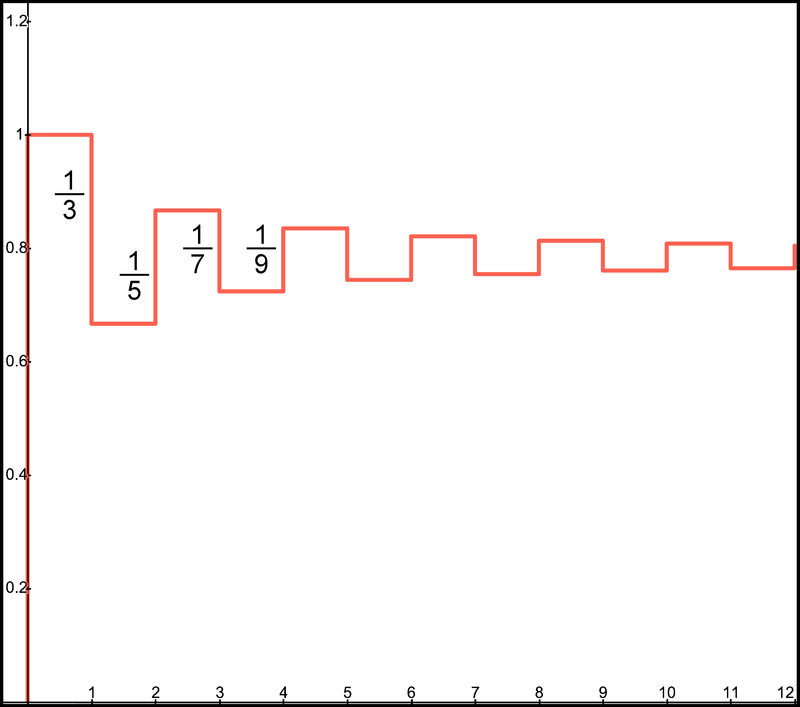
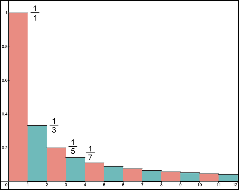
The graph in Figure 1 shows the cumulative sum as we add another term left to right. The $x$-axis represents the number of terms in the sum. The shape of the graph looks like stairsteps similar to the harmonics series. However, because the terms have alternating signs, the steps have an up and down pattern.

Our logical question is: What number does this sum approach?

Target shooting

If you view Figure 1, clearly the result is moving toward a fixed number, a target if you will. Think of this infinite sum approaching some target or bullseye. When we add one more term, the sum gets closer to the bullseye. The first shot is 1 and overshoots the target. We add a second term to the sum to lower our aim by $\frac{1}{3}$, so our second shot is at $\frac{2}{3}$. But we go too far, and we undershoot the target. However, the good news is, after the second shot, we are closer. Since we’re below the target after 2 shots, add another term that will raise the target by $\frac{1}{5}$. Thus, our third shot is $\frac{2}{3} + \frac{1}{5}$ or 0.8666. Again, we overshoot, but again we get closer. Then, we lower our aim by $\frac{1}{7}$ and shoot again with the number $0.86666 -\frac{1}{7} = 0.7238$. We keep this process of making our next aim better than the previous aim, but we always go a bit too far and overcompensate. However, as long as we continue, we keep getting closer to the bullseye.

With our next shot, which is our fifth shot, we’ll add $\frac{1}{9}$ and get this random-looking, uninteresting number: 0.83492. Since we will subtract the next number, then our sum will be less than 0.83492.  Jumping ahead after 10 shots, we get to 0.76046, a number that's still random-looking, still not interesting, but we are closer to the target. Where will this musical chairs of addition and subtraction end? I’ll give you a clue: the target number we will identify is irrational. Remember we cannot completely write an irrational number because it has an infinite number of digits.

Of course, our goal is to identify which irrational number it is. We already learned that there are actually more irrational numbers than rational numbers, so we have a lot to choose from. Most irrational numbers are not interesting. However, I wouldn’t be sharing this if it didn’t have a happy ending. Perhaps there is another mystical (transcendental?) number out there between 0.76046 and 0.83492.

The answer

The sum of this infinite series within 15-decimal precision equals 0.785398163397448. What does it equal exactly? It exactly equals $\frac{\pi}{4}$.

I consider this an amazing result. It’s not only significant to me; it actually shocked the math community in the day it was discovered. The guy who is famously credited for finding this connection is Gottfried Wilhelm Leibniz. Yes, this is the same guy who co-authored calculus. I think this formula has made a major impact on the math we know today. Leibniz published this series in 1676 just as he began his work in calculus (end of 1675). It seems likely this boosted his confidence in doing math.

The story goes that Leibniz thought he found the secret of nature when he uncovered this formula. It was a turning point in his life. He was a lawyer and diplomat when he decided to quit his day job and pursue mathematics full time. Leibniz made great use of his new profession as he co-authored calculus along with Isaac Newton. We can speculate that Leibniz influenced calculus more than Newton because when he was publishing about calculus, he was thinking about how to make calculus useful for others. He created wonderful notation that is still used today. In contrast, Newton used calculus more to solve his physics problems. What Newton did was truly amazing, but his version of calculus didn’t relate well to the masses, so Leibniz is the primary person who has influenced the calculus we know today. From one perspective, we can state that this problem has had a significant impact on our current calculus because of the story of how it impacted Leibniz and how Leibniz then impacted calculus. From this perspective, we could state that Leibniz created the "process" of calculus because he was able to “package” his ideas using useful notation. With that historic backdrop, let’s return to our problem.

Because $1 - \frac{1}{3} + \frac{1}{5} - \frac{1}{7} + ...$ is equal to $\frac{\pi}{4}$, we have another way to calculate $\pi$. We can approximate $\pi$ simply by including as many terms in this sum as we want, then multiply the result by 4. It takes a while, so it is a difficult way to estimate $\pi$. In fact, you must include 10 million terms to estimate $\pi$ accurately to 8 decimal places. Slow, indeed.

However, the benefit for calculating $\pi$ by different methods is not a game of precision but vision. Sure math people make a sport of it, but that is not the primary benefit. We as humans like to push boundaries, so calculating more digits of $\pi$ stretches those boundaries even if it doesn’t add significant value to even the math community. Eight decimal place accuracy is sufficient for almost every possible practical need for $\pi$. Three or four decimal places will usually suffice. But our focus in Lazarus Math is the journey, not the destination. So we can benefit from the process of finding different ways to calculate $\pi$ because it may enlarge our vision and give us a different perspective. Often, it is the method that we uncover to calculate $\pi$ that can be of value. This was certainly true for Leibniz when he developed this formula. This was the first calculation of $\pi$ that was written as an infinite series. That may not seem important, but it was a milestone in math when it occurred.

I find it interesting that many of the great minds of math have put forth significant effort to uncover some of the properties of $\pi$ by creating some new process. Just a small list of names include Archimedes, Descartes, Newton, Leibniz, several Bernoullis, Euler, Gauss, and the list goes on. Perhaps it may help to see the significance of this with a painting analogy.

Imagine if many of the great painters of history worked together on a collage type painting that somehow blended together to create something special. This certainly has the potential for being special. Counting the total number of brush strokes made by all the painters might measure some sort of quantity of output, but it would not be the best measure of its importance. What would be more important is what they painted.

Likewise, these great math talents added to the precision of $\pi$, but that is like counting paint strokes. Rather, what is important is all the creative work they invested in the process of working with $\pi$ that has paid huge dividends to the math community. They have discovered new principles and methods through their creative work.

An area of opportunity

What I’ve shared about the Leibniz series so far is common knowledge. But in writing Lazarus Math, I try to consider results from different perspectives. So I thought about this result and I found some ideas that seemed interesting, at least interesting to me. As usual, some of the thoughts in these stories are just my notions that I’m sharing for you to ponder.

Let’s start with our result. I find it fascinating that the result is an irrational number. Notice we are just adding a simple function of the odd integers where each term clearly is rational. I wonder at what point in the sum it becomes irrational. My hunch is that it only becomes irrational when we travel to infinity. In other words, my hunch is if we stop the sum at some finite number of terms, the result would be rational. Perhaps one of the Lazarus Math readers can share insight into my hunch.

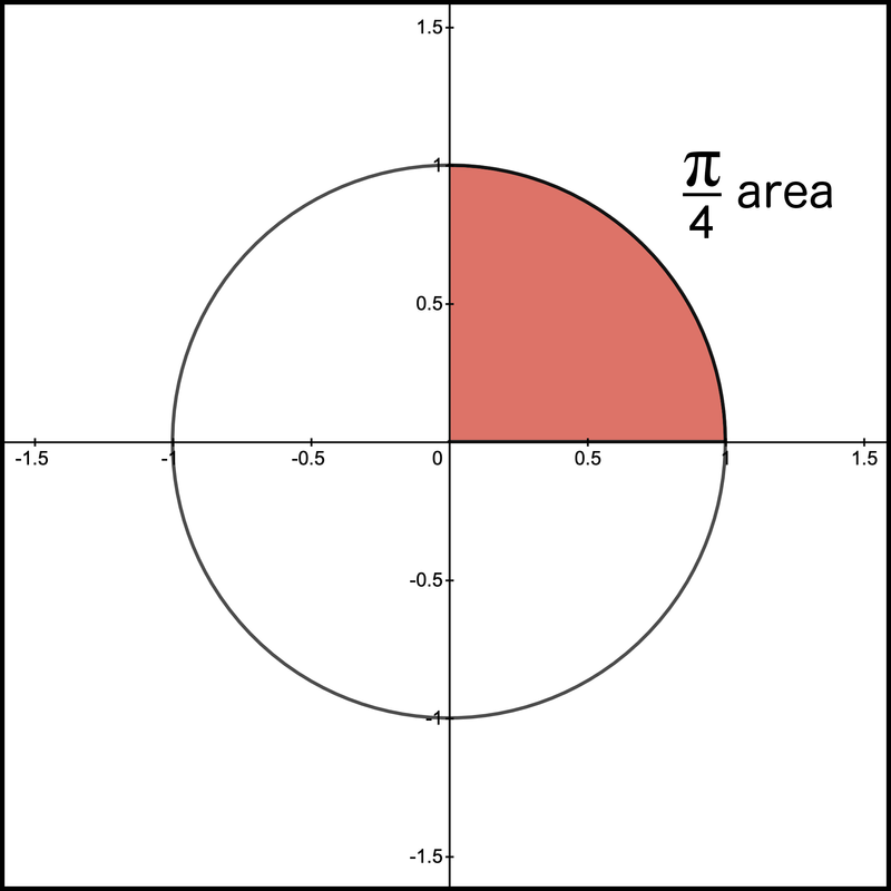
Perhaps more interesting is how we view the result. We landed on the number $\frac{\pi}{4}$ as the sum of our infinite series. Another way we can picture this result is not as a number but as an area. We’ve been down this path before, so thinking of a number as an area is expected but perhaps not for this problem. Recall the area for a circle is $\pi r^2$. The unit circle has radius $r = 1$, so its area is $\pi$. It may seem strange, but we can view the sum of this infinite series as the area of $\frac{1}{4}$ of a number circle as illustrated in Figure 2.

Isn’t that interesting? It seems almost bizarre to connect the sum with this area. Yet, both produce the same result. What do we make of this perspective? Is there any connection between the two perspectives? By now, you likely can guess our next questions: Why does $\pi$ show up? How is this sum equal to the area of $\frac{1}{4}$ of a unit circle? This is worth thinking about. The special number $\pi$ is always tied to something round. How could $\pi$ make an appearance in a recipe that only involves odd integers? If someone gave you a problem and asked: How can the odd integers relate to $\pi$? You likely would answer they don’t. Yet they do. We know this is not just a coincidence. What is the connection? Are you curious to learn? Where would we even begin to write this story if we started with a blank sheet?

Area from rectangles

Let’s start with a blank sheet and see if we can narrate a story. It was quite easy to view the total for the sum, $\frac{\pi}{4}$, as an area since it is the area of $\frac{1}{4}$ of a unit circle. Let’s consider the infinite sum as an area as well. We’ve actually already started down this road. Recall our original stairstep graph. Rather than show the net effect after each new term, we can create the area for each term. If a rectangle has a base of 1, then its area will be its height since the area of a rectangle is the base (which is 1) times the height. We’ve used this clever technique before. We think of a number as an area by creating a rectangle with length 1 and its height as the number we are representing. Then, we organize these rectangles on the $xy$-coordinate system. Even though we are just beginning, we are going down the same path we have travelled with other math problems. So this start should be familiar territory.

Our first term is 1, so let’s think of 1 as an area of a rectangle. Using a base length of 1, create a rectangle, actually a square, that has a height of 1 to represent an area of 1. The next number in our sum is $\frac{1}{3}$. Convert the number $\frac{1}{3}$ to an area $\frac{1}{3}$ by creating a rectangle with height of $\frac{1}{3}$ and base 1. Because of the alternating signs of the terms in the series, we must visualize subtracting the area for the rectangles representing every even term in our sum. Thus, imagine subtracting rectangles that have area $\frac{1}{3}$, $\frac{1}{7}$, $\frac{1}{11}$, etc., which are the teal rectangles in Figure 3. Again, the vertical and horizontal axes are not the same scale.

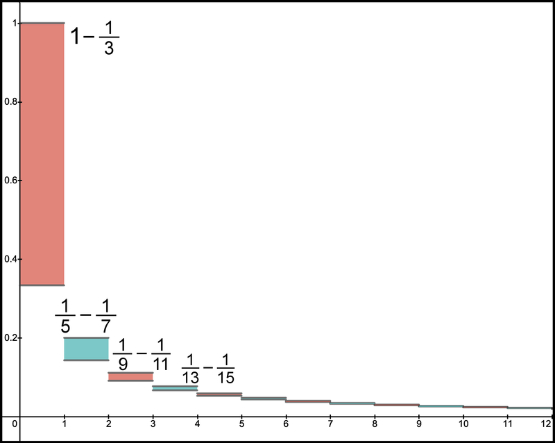
We can imagine subtracting an area by pairing the negative number with the previous positive number. In other words, pair the positive 1 with the negative $\frac{1}{3}$. The graph in Figure 4 shows the difference between successive positive and negative terms. Now, think of the net area from each pair as what we are adding. Thus, the total sum is the sum of the areas for each net difference. Notice the $x$-axis now represents a pair of numbers. The range from 0 to 1 represents the first pair, the range from 1 to 2 represents the second pair, etc. Thus, $\frac{1}{13}-\frac{1}{15}$ is the 4th pair and represents the area for the 4th pair of integers. It is clear that the first few rectangles here have decreasing areas as we move left to right. Even though the last several rectangles appear to be about the same size, they are actually decreasing in area.

Isn’t this an interesting way to view a sum that has alternating signs? Hopefully, this is a clear picture of the area for this infinite sum. However, we haven’t made progress identifying how this connects to the area for $\frac{1}{4}$ of the unit circle. We are on the right track by viewing differences in areas between successive terms. How can we arrive at the finish line, which is $\frac{\pi}{4}$? This is a good start. However, rectangles are straight, and we know $\pi$ relates to a circle. So how do we go from something straight to something that curves?

Area from curves

The idea is to follow a similar strategy of using area but using curves rather than rectangles. Like before, start with the infinite series $1 - \frac{1}{3} + \frac{1}{5} - \frac{1}{7} + ...$. Remember the width of the base for the rectangle is always 1. We will follow the same strategy for our curve solution. However, this time we will assume the range for each curve is always between $x = 0$ and $x = 1$. It will be easier to understand this curve approach as we step through the details.

Previously, we envisioned our area by stacking rectangles left to right. Now, we will envision our area by stacking curves on top of each other within this range of $x = 0$ and $x = 1$. All we are doing is shifting the areas to the same range between $x=0$ and $x=1$. So the width of each area remains 1. Now we need to match the total area with a curve that has the same width.

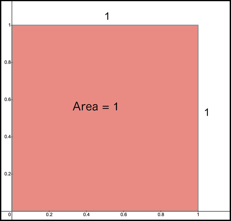
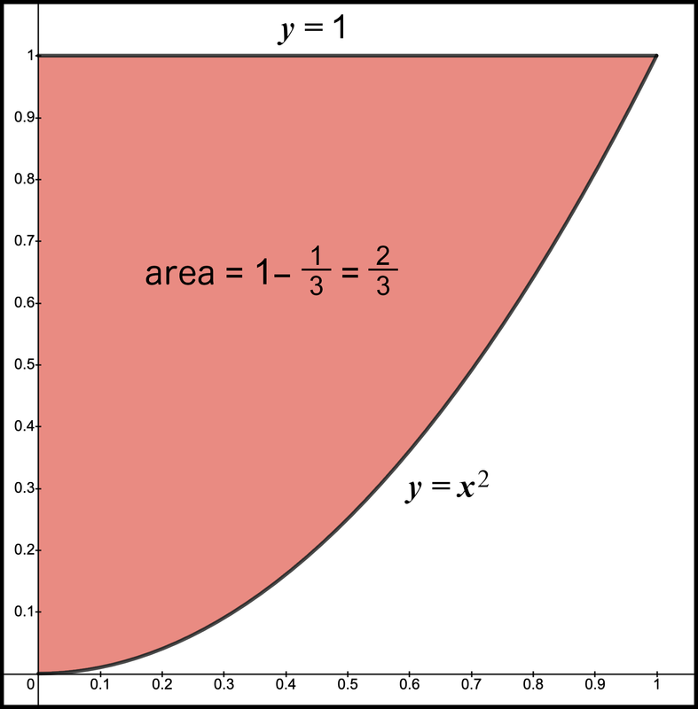
We will eventually combine the positive term with the negative term and view the net area. But first, let’s review the area for each term. Our first goal is to reproduce the number 1 with a shape within the range of $x = 0$ to $x = 1$. For the first number, we will not get creative but instead retrieve our rectangle solution by using a rectangle with height 1. Since the base and the height are both 1, we actually created a square. Figure 5 is our area for the number 1. No surprise yet. Let’s hint at our creative process by thinking of 1 as $1^0$ since any positive integer raised to the power 0 is 1.

Next, we need to create a shape with area equal to $\frac{1}{3}$, also between $x = 0$ to $x=1$. Sure, we could create a rectangle that has height $\frac{1}{3}$ and base 1, but our goal here is to use curves. This leads to a rather interesting question. What is a definition for a function such that the area below the function, above the $x$-axis, and between $x = 0$  and $x = 1$, equals $\frac{1}{3}$? There likely are many graphs that achieve this criteria but we are heading to a specific target, so the graph we want is $y = x{^2}$.  You may wonder how I know the area under the graph of $y=x^2$ between $x = 0$ and $x = 1$ is $\frac{1}{3}$.

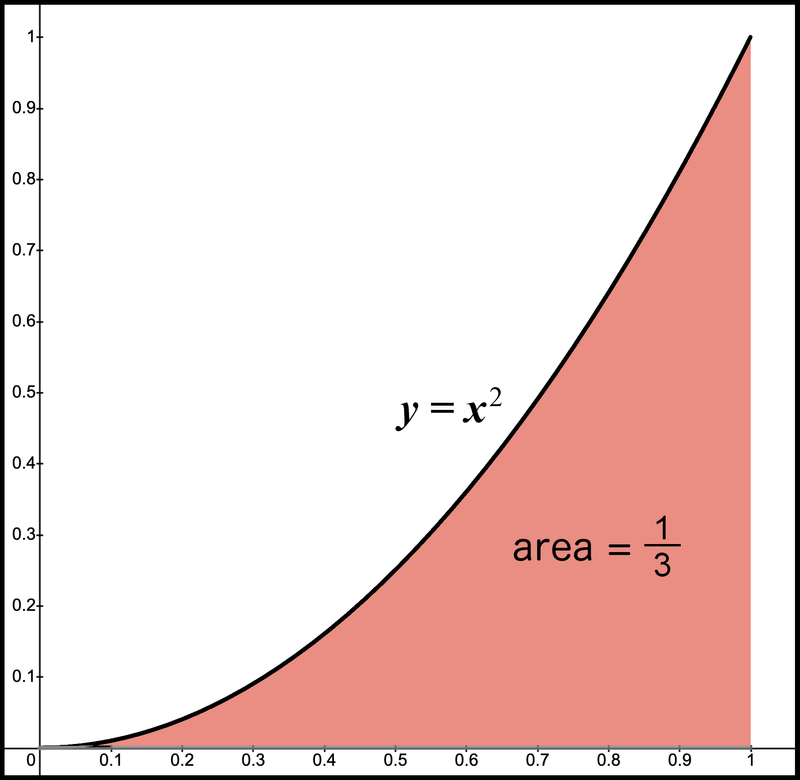
Let’s start by reviewing Figure 6 to visualize the area. We want to calculate the area under the graph of $y = x^2$. Intuition would lead me to think the area is some random number, not a nice fraction such as $\frac{1}{3}$. But, how do we calculate this area? Fortunately, this seemingly impossible task has been solved by calculus. I’m assuming you have not studied calculus. However, this idea is so amazing I want to pause and explain the details. Even though we will use calculus to calculate several areas, they all follow one pattern. Thus, we just need to understand one process and then repeat it.

We begin the process by rewriting the output of the function $y = x^2$ by increasing the exponent by 1 and dividing by the new exponent. That means $x^2$ becomes $\frac{x^3}{3}$. We can call this the area graph for the original function.

Notice we actually have two functions at play. We have the original function for which we want to calculate the area, and this function is $y = x^2$. Then, we have the area function that is the solution to the area question (area function = $\frac{x^3}{3}$). In other words, the answer to the area of a function is another function. Then, we manipulate the area function to calculate the area of the original graph because we want a specific number for an area, not just a function of $x$. How do we convert this function of $x$ to an exact number? Here’s our recipe for calculating the area using our area function.

Calculate the area under the graph between 0 and 1 by first substituting 1 for $x$ into our area function $\frac{x^3}{3}$. Then, do it again but substitute $x$ for 0. Take the first result minus the second result. Notice these numbers correspond to the range we are working with. This gives us the area under the graph of our original function $y = x^2$. That means the area under the graph of $y = x^2$ between 0 and 1 is $\frac{1}{3}$ - $\frac{0}{3}$ = $\frac{1}{3}$.

Observe we used this process for our first number. We can think of the graph of $y=x^0$, which is the same as $y=1$. Then we can reproduce this area by following the pattern we just uncovered. The area function is $y=\frac{x^1}{1}$. Thus, substitute in 1 and 0 for $x$ to get $1-0=1$, matching our original result.

Very good. We just produced a shape that has an area of 1 and another shape that has an area $\frac{1}{3}$. Remember in our infinite sum, 1 is positive and $\frac{1}{3}$ is negative. The next step is to combine the positive and negative areas similar to what we did with the rectangles. Figure 7 is a picture where the shaded region represents the first area minus the second area.

Since the area of the first graph is 1 and the area of the second graph is $\frac{1}{3}$, then the difference in the area of the two graphs must be $\frac{2}{3}$. Thus, the area of the shaded region is $\frac{2}{3}$ or, more importantly, $1 -\frac{1}{3}$. We are able to calculate this net area because both areas range from 0 to 1. Not only do they cover the same range, but the area under the graph of $y = x^2$ is a subset of the area of the square within this range. We will see this concept repeat for each pair of terms where the negative term we are subtracting is a subset of the positive area we are adding.

Repeating the process

This is heavy math and it may take a while to let it sink in. When you are ready, we will just repeat this process. If you enjoy challenges, you may try to reproduce the result for the next two numbers on your own. Even though we have only performed the math on the first pair of integers, doesn’t the shaded area in Figure 7 resemble the area for $\frac{1}{4}$ of a circle. Isn’t that significant progress? We have jumped the gap from straight things to curved things!

OK, our next step is to look for the graph of a function whose area is $\frac{1}{5}$ within the range 0 and 1. Again, we can use the magic of calculus to identify the function we need is $y = x^4$. Figure 8 is the graph of this function with the area shaded between 0 and 1.

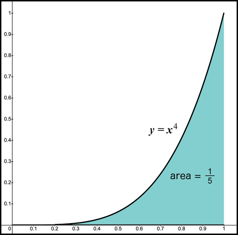
How do we know that the graph $y = x^4$ produces the area we need? Like before, we take the original function and identify the area function. Our recipe to identify the area function is to increase the exponent by 1 and divide by the exponent. This produces the area function $\frac{x^5}{5}$. Again, substitute 1 for $x$ and 0 for $x$. Take the result when we substitute 1 for $x$ and subtract the result when we substitute 0 for $x$ to get $\frac{1}{5}$ - $\frac{0}{5}$ = $\frac{1}{5}$. Don’t worry if this still seems difficult. It literally took the math world thousands of years to discover this pattern. However, it is truly one of the greatest moments in math history.

So far, I have given you the function we need and then calculated the area function from that function. With a couple of practice rounds completed, we are ready to fully reveal the process so we can produce the results for other numbers. Assume we are given an odd integer $n$. We identify our initial function by subtracting 1 from our number and then raising it as an exponent. In general, our function would be $y = x^{n-1}$. This is because we create the area function from $x^{n-1}$ by raising the exponent by 1 and dividing by the exponent. This means our area function is $\frac{x^n}{n}$. Then, when we substitute 1 for the first term, we always get $\frac{1}{n}$, and when we substitute 0 for the second term, we always get 0. Thus, the area is always $\frac{1}{n}$ - $\frac{0}{n}$ = $\frac{1}{n}$, which produces the fraction we want for a given number $n$.

As a side note, you may wonder if this recipe always works. What happens if we input a negative integer? Does it work for real numbers? This recipe works not only for integers but for all real numbers, not just the positive real numbers but the negative real numbers. There is only one exception, and we have identified this exception earlier in Lazarus math. The only exception is if we apply this process for $n=0$. If we followed the recipe for $n=0$, we would get a result $\frac{1}{0}$, which is not defined. Also, if we followed this pattern, then our original function would be $y = x^{n-1}= x^{0-1}= x^{-1}=\frac{1}{x}$. Remember we identified the area function for this function is the natural log function. If all of this isn’t slick, I’m not sure what is! We have this wonderful process that works for all real numbers except one. That one exception happens to be the definition for the natural log function. Maybe you have had calculus. Have you thought about this before?

If you want to know why this pattern works, you are a great candidate to study calculus! Please be sure you understand this pattern before we continue.

Wonderful. Now, we know our recipe, let’s quickly cook the remaining part of our solution.

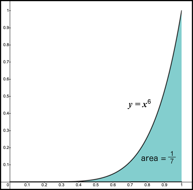
The next number we need is $\frac{1}{7}$, and the graph that provides an area of $\frac{1}{7}$ is $y = x^6$ as illustrated in Figure 9.

Remember $\frac{1}{5}$ is positive and $\frac{1}{7}$ is negative, so pair these two graphs by taking the positive result for the first graph and subtracting the result for the second graph. Thus, the area of the difference, $\frac{1}{5}$ - $\frac{1}{7}$, is the area in the shaded region of Figure 10. Again, the area under the graph of $y = x^6$ is a subset of the area under the graph of $y = x^4$. Thus, when we take the difference between the two areas we can start with the larger area and remove the smaller area to show the net area.

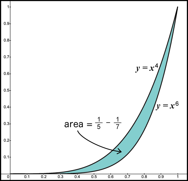
Let’s repeat this process once more. We now want a graph whose area between 0 and 1 is $\frac{1}{9}$. Calculus indicates the function we need is $y = x^8$, and the graph that provides an area of $\frac{1}{11}$ is $y = x^{10}$. Figure 11 shows graphs of both together.

As before, all of $y = x^{10}$ is contained in $y = x^8$. You may wonder why the negative area is always a subset of the positive area. We’ve glossed over this concept, so let’s think about this for the numbers 8 and 10. Because our range is between 0 and 1, when we multiply the number by itself, the result always decreases the more times we repeat the multiplication, except for the endpoints 0 and 1. As we increase the exponent, all results between 0 and 1 will be smaller if the exponent is larger. Thus, $x^8$ is larger than $x^{10}$, except at the endpoints 0 and 1 where they are the same. That means if we view this graph and want to know the area under $y = x^8$, we include the top part, which has the darker shade, and the bottom part, which has the lighter shade. Then, when we take the difference, we only include the top part. We know the area under the graph in Figure 12 between $x = 0$ and $x = 1$ is $\frac{1}{9}$ - $\frac{1}{11}$.

This pattern is the same for all pairs of numbers we consider. This is because the positive area always contains the entire area we subtract since we are considering the interval between $x = 0$ and $x = 1$, where a smaller exponent produces a larger number. This is just one more fascinating nugget in this story.

Of course, if we traveled to the landscape where $x$ is greater than 1, then the reverse is true and the function with the larger exponent will always be greater. But we’re restricting ourselves to between 0 and 1 where the function with the smallest exponent is always the largest number.

A captivating harp

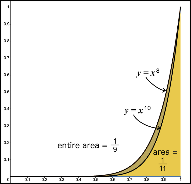
Let’s review our 3 results so far. By taking the positive term and subtracting the negative term, we have produced the following areas in Figure 13.

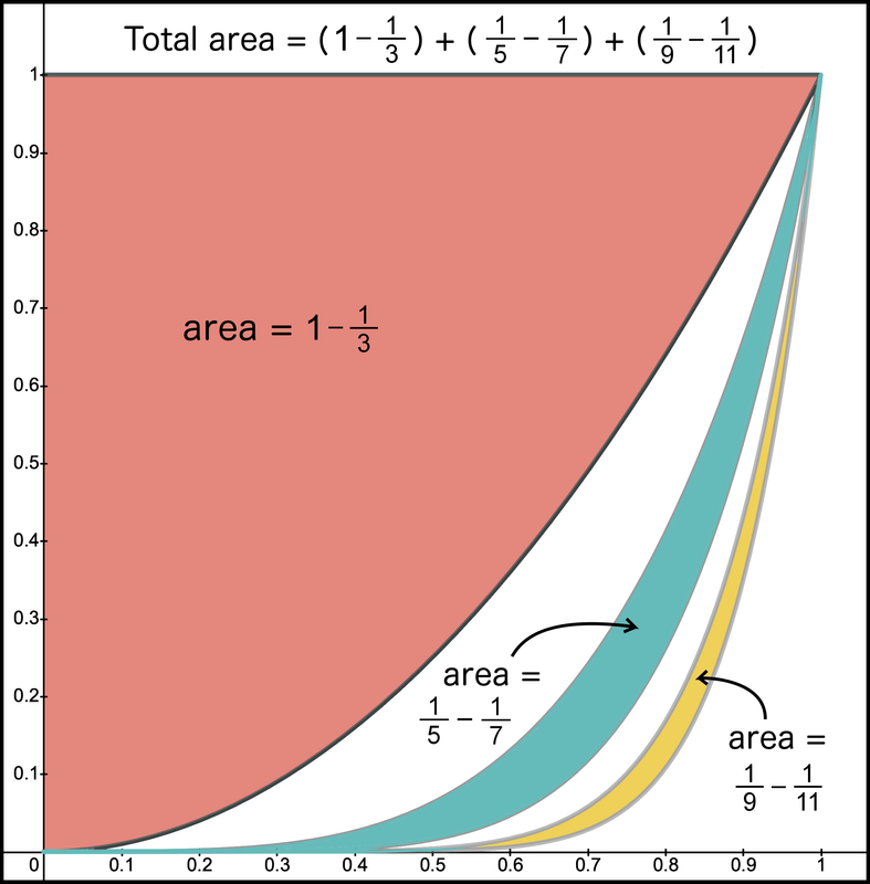
If we want the area for all 3, we can sum the areas of each piece. The area for the largest piece is $1 - \frac{1}{3}$, the area for the next largest piece is $\frac{1}{5}$ - $\frac{1}{7}$, and the area for the smallest piece is $\frac{1}{9}$ - $\frac{1}{11}$.

We created each of these by following a pattern. We can repeat this pattern, in theory, forever. Figure 14 is a picture of the first 3 and the next 3 shapes, or net areas.

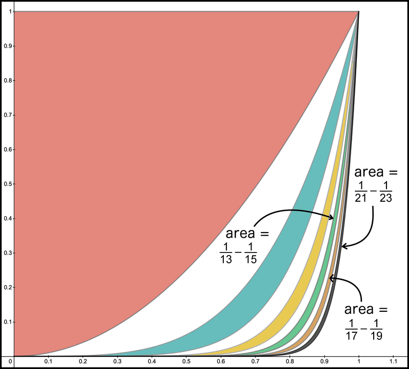
The net area for the next 3 pieces follows the same pattern: $\frac{1}{13}$ - $\frac{1}{15}$, $\frac{1}{17}$ -$\frac{1}{19}$, and $\frac{1}{21}$ - $\frac{1}{23}$.

In summary, we’ve created a process that reproduces our integer sum. You must admit, it is a pretty way to visualize this infinite sum. Much more beautiful than just a bunch of numbers smashed together, and even better than comparing rectangles.

But all we’ve done is find an artistic way to write our sum. We’ve introduced some curves, but how does this yield the result $\frac{\pi}{4}$? Currently, this picture resembles a fancy harp more than $\frac{\pi}{4}$. This has been a long journey so I appreciate your staying with me thus far. Surprisingly, we only need two imaginative steps to get us to the finish line.

Another equal area

Our first step is to rewrite what we did on the graph in algebraic form. We identified that the infinite sum ($1 - \frac{1}{3} + \frac{1}{5} - \frac{1}{7} + \frac{1}{9} - ...$) is the same as the area under the graphs of $y = 1$ minus $y = x^2$ plus $y = x^4$ minus $y = x^6 ...$ between the interval of $x = 0$ and $x = 1$.

So, let’s combine these functions into one expression and maintain the correct signs. The first shaded area started with the function $y = 1$, then we calculated the net area by subtracting the area from the function $y = x^2$. We can combine this into one function and say $y =1- x^2$. Likewise, we can rewrite the net area for the second part as $y =x^4-x^6$. The function for the net area for the third piece is $y =x^8-x^{10}$, and so on. Then, there is no reason why we cannot combine all these areas. Thus, the total area for the first 6 shaded regions is the area between 0 and 1 of the function

This only includes the first 6 pairs, but the sum we are after is an infinite sum. We can make this sum an infinite sum by adding the 3 dots afterwards, indicating this pattern continues forever.

What type of infinite sum is this? For example, if we know the first 5 terms of the sum, how do we determine the 6th term? Notice we can identify the next term by taking the previous term and multiplying by $x^2$. However, since the terms have alternating signs, the exact factor is $-x^2$. In other words, start with 1 and multiply by $-x^2$. The result is $-x^2$. Then, take this term and multiply by $-x^2$. The new result is $+x^4$. Again, multiply by $-x^2$ to get $-x^6$, and so on. Does this type of a series resemble anything we studied? We just learned about this type of series. This is the sum of a geometric series. We know it’s a geometric series because we can create the next term by taking the previous term and multiplying it by some factor. Here, this factor isn’t a constant but involves $x$. However, the factor is the same each time and the operation to generate the next term is multiplication, so this is a geometric series. Isn’t it neat when you learn one trick in math and you can immediately apply it to a totally different problem? Do you see why it was useful to understand a sum of a geometric series? It is a process that occurs a lot in math. Also, we just expanded our notion of this geometric series to apply to variables in addition to constants.

Since we have a formula for this sum, let’s retrieve and reuse. Recall the formula is the first term divided by (1 minus the common ratio). Here, the first term is 1 and the common ratio is $-x^2$. Remember our common ratio must be greater than -1 and smaller than 1. Since we are only viewing the range between 0 and 1, we achieve this condition. Next, substitute these numbers to get:

$$\text{Sum}=\frac{1}{1-(-x^2)}$$

Since subtracting a negative value is the same as adding a positive value, our sum simplifies to the beautiful $\frac{1}{1+x^2}$. Wow. That formula sure came in handy. We just condensed an infinite sum into a rather simple fraction. Of course, it doesn’t look like the two should be related but that is par for the course in math!

OK, that was step 1.

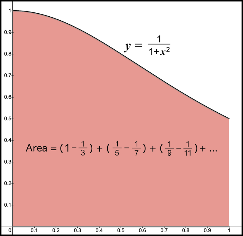
What does step 1 tell us? It tells us that the area under the graph of the infinite sum between 0 and 1 is the same as the area under the graph of $y=\frac{1}{1+x^2}$.

They must have the same area for the same region since their expressions are mathematically identical. This isn’t obvious if we just compare their areas in Figure 15. Because we have a new function that is mathematically equivalent to the previous function, the areas may look different but they will match within our range. We can trust the formula for the sum of a geometric series not to lead us astray. Yes, we still don’t have our result, but this is only step 1.

What step 1 also tells us is the area of this graph between 0 and 1 is the same as the area of our infinite slices, for which we only drew the first 6 slices in Figure 16.

Thus, even though the region in Figure 15 looks very different from the region in Figure 16, we know they have the same area by using the formula for the sum of a geometric series.

π finally appears

What is step 2? Step 2 gets us to the finish line as we try to calculate the area under the graph of $y = \frac{1}{1+x^2}$ between $x = 0$ and $x = 1$. The area of this graph, like many graphs, looks difficult to calculate. Previously, when we wanted the area of a curved graph, we’ve turned to calculus to bail us out. Does calculus have a magic bullet here?

In fact, it does. A rather obscure bullet, but it does the job perfectly. Remember the way calculus gives us the area under a function is not a numeric answer but another function. So, our next question is: What is the area function connected to the function $y=\frac{1}{1+x^2}$?

The previous examples we considered were polynomials and we identified the rule for polynomials. This function is not a polynomial, so we need another rule. This rule has a surprising ending.

Believe it or not, the function we need is connected to the sine and cosine function. You may recall from trigonometry what you get when we take the ratio of sine to cosine. The ratio of the sine function to the cosine function is the tangent function. In other words, the tangent function is simply the sine of an angle divided by the cosine of the same angle. We go one step further into obscurity because the function we need isn't the tangent function, but it is related to the tangent function. The function we need is called the inverse tangent function. In math, when we see the word "inverse," we think of "opposite" or "undoing". Let's learn how the inverse tangent function is the "opposite operation" of the tangent function.

For example, the tangent of an angle measuring 45 degrees is 1 if we measure with degrees. Or, we can also use radians. Remember a full circle is $2\pi$ radians. Since 45 degrees is $\frac{1}{8}$ of a circle, then 45 degrees is equal to $\frac{\pi}{4}$ radians. Thus, the tangent of $\frac{\pi}{4}$ radians is 1. Then, when we apply the inverse tangent, we switch input and output. That means the inverse tangent of 1 is $\frac{\pi}{4}$ radians. In other words, the inverse tangent function does the job its name promises. It takes the inverse or undoes what the tangent function does.

How does the inverse tangent function help here? It just so happens that the area under the graph of the function $y =\frac{1}{1+x^2}$ within any interval on the $x$-axis is the inverse tangent evaluated at the ending point minus the inverse tangent evaluated at the beginning point. Thus, the magic wand of calculus gifts us the interesting solution that the area under the graph of $y = \frac{1}{1+x^2}$ between the points $x = 0$ and $x = 1$ is the inverse tangent of 1 minus the inverse tangent of 0. Even though we had a different way to derive our area function than we did with the polynomials, we still followed the process of evaluating the result at $x=1$ and subtracting the result at $x=0$. So the only thing new in step 2 is identifying a different area function.

Remember, we just identified that inverse tangent of 1 is $\frac{\pi}{4}$. Also, the tangent of 0 radians is 0, so the inverse tangent of 0 is 0. Combining the two produces the result $\frac{\pi}{4}$ minus 0, which allows us to finally arrive at our destination, $\frac{\pi}{4}$.

That was some conclusion! It’s been a long journey, so let’s summarize.

Summary

Our initial goal was to calculate the sum of $1 - \frac{1}{3} + \frac{1}{5} - \frac{1}{7} + ...$

We changed dimensions from 1 to 2 by converting numbers to area. First, we created a series of rectangles whose area matched the result of the infinite sum. This was a good start in using area in the solution, but it didn’t help connect the sum to $\pi$. Thus, we tried a similar technique except we used curved shapes instead of rectangles to calculate the area. The function that we identified that had the same area as our infinite sum is the area under this function above the $x$-axis and between $x = 0$ and $x =1$:

Since this is the sum of a geometric series, we know that this infinite sum can be rewritten using the formula for the sum of a geometric series:

Because these two are equal, then we know that the area under this new function must also equal our infinite sum. We know from calculus, the area function connected to the function $y =\frac{1}{1+x^2}$ is the inverse tangent function. That means the area under the graph $y =\frac{1}{1+x^2}$ between $x = 0$ and $x =1$ equals the inverse tangent of 1 minus the inverse tangent of 0. Since the inverse tangent of 1 is $\frac{\pi}{4}$ and the inverse tangent of 0 is 0, our infinite sum is $\frac{\pi}{4} - 0 = \frac{\pi}{4}$.

Going full circle

As I marveled at what we uncovered in this wilderness journey, I still gave this problem more thought and made another observation. If you recall, we started our research by recognizing the area of $\frac{1}{4}$ of a unit circle equals $\frac{\pi}{4}$ . Figure 17 shows the same circle.

It is interesting to see how our infinite sum completes the area for the quarter of a circle as we add positive net terms. Figure 18 shows the area added for each positive net term. The colors for each area are consistent with the colors in Figure 16. We show the area for the integers up to 23. You can see how much of the quarter circle remains unshaded after each new sum is added.

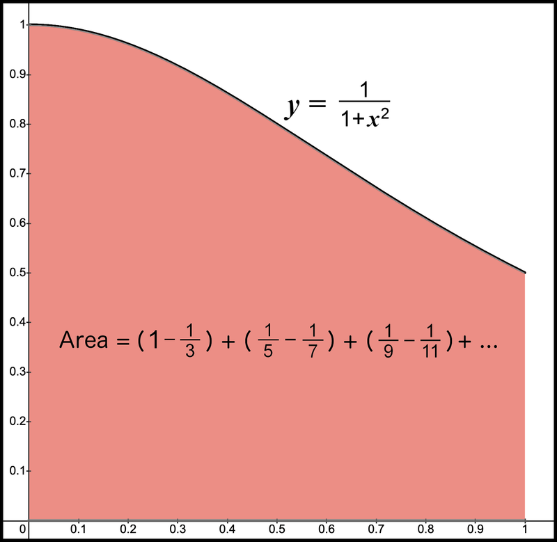
Eventually, we identified that this also equals the area under the function $y =\frac{1}{1+x^2}$ above the

$x$-axis and between $x=0$ and $x=1$. Figure 19 is the same graph for this function we viewed earlier.

I will call this our solution function since this is the final function that produced the area we were after.

Notice both of these graphs are bounded above by $y=1$, below by $y=0$, to the left by $x=0$, and to the right by $x=1$. We also know the area under each of these graphs within these boundaries are the same. Both equal $\frac{\pi}{4}$. Since these two graphs equal the same thing, let’s review the two graphs together.

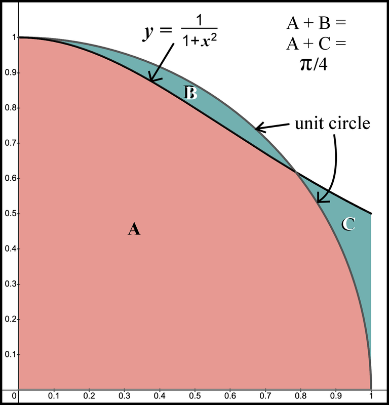
Figure 20 shows three shaded regions: A, B, and C. A is the area included in both the graph of the unit circle and the graph of $y=\frac{1}{1+x^2}$. B and C are areas that are unique to one of the graphs. The area unique to the unit circle is labeled B, and the area unique to the solution function, $y=\frac{1}{1+x^2}$, is labeled C. I will remove the shading for A to focus on the areas that are different in Figure 20.

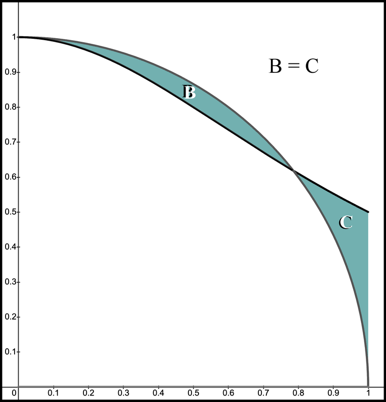
The total area between $x = 0$ and $x=1$ for the unit circle and for the solution function both equal $\frac{\pi}{4}$, and the common area A for each is the same. That means the areas that are not common to each must also be the same. The long thin area on the left (labeled B) is the part of the circle that is not part of our solution function. The thicker and shorter area on the right (labeled C) is the area that is part of our solution function but is not part of the circle.

Even though these two areas have different shapes, we know they have equal areas. We know this because $A+B = \frac{\pi}{4}= A+C$. Therefore $B=C$. In case you are curious, the area $B=C+0.0290$, which means $A =\frac{\pi}{4} - 0.0290 = 0.7564$ to 4-decimal precision.

Tricks of math

One of the neat things about math is all the tricks we have up our sleeve. This problem started as the sum of an infinite series connected to odd numbers. If you want, we can think of this as a one-dimensional problem, such as a number line. However, in our solution, we increased the dimension from 1 to 2 and viewed the problem from an area perspective. Then, we used the tools and techniques that we have for calculating area, namely calculus, to arrive at the conclusion in two dimensions that matched the result we proposed in one dimension. This is no small task.

A main pursuit of math people is developing systems that produce consistent results. We wandered way off our path into the calculus world and recycled the inverse tangent function to calculate area. Even though our problem did not involve angles, we are confident that the math is consistent when applied correctly to angles, numbers, and areas. Because calculus has such a rich library of ways to calculate areas, it becomes a favorite resource to solve problems.

In many respects, it may have appeared we were going down the wrong path because we made the problem more complicated. After all, we only wanted to add and subtract numbers. Yet, we wandered off to technical calculus tools in order to get us to the finish line. Much of math is not only discovering new things but how these new things are connected, often surprisingly so, to things we already knew, such as a sum of a geometric series. As a result, we have a much broader scope of tools and techniques to work with to solve new problems. It’s like getting a new tool to solve a problem and not only learning the benefits of the new tool but realizing it makes the existing tools you already own even more valuable.

I hope this solution stirred something inside you. The answer was certainly interesting. But how we arrived at the answer is captivating, at least to me.

Historical note

We often write the inverse tangent of $x$ as $arctan(x)$. With that, we have the Leibniz series:

$$arctan(1)=\frac{\pi}{4}= 1- \frac{1}{3} + \frac{1}{5} - \frac{1}{7} + ...$$

However, we have a more general version of this series that was first credited to Madhava of Sangamagrama (1350-1425), who lived a couple hundred years before Leibniz. Here is the more general version.

$$arctan(x)=x - \frac{x^3}{3} + \frac{x^5}{5} - \frac{x^7}{7} + ...$$

We also refer to this general series as the Gregory series after James Gregory. Gregory published this general series a few years before Leibniz published his series, where Leibniz made the rather trivial substitution of $x=1$. Gregory’s publication is the first publication that has survived whereas Madhava’s work has not and is only referenced by other writers.

Madhava’s story is important because he is a pioneer of understanding how to bring infinity to math. This is a key theme in Lazarus Math and a remarkable feat for someone who was born in the 14th century.