Big Becomes Beautiful

“[Imaginary numbers are] a wonderful flight of God’s Spirit; they are almost an amphibian between being and not being.” Gottfried Leibniz

Reviewing Euler’s equation

Are you enjoying living life in the complex plane? In the first section for the New Dimensions portion of Lazarus Math, we covered the basics of how to do math in the complex plane. In the second section, we witnessed one of the most beautiful equations in math, often labeled as Euler’s equation. The beauty was clearly revealed when we observed the output on the complex plane. Books have been written about this equation highlighting all its beauty.

Aside from the beauty, there is a key takeaway from the previous section I want to highlight. The key takeaway was when we changed the input from $x=2$ to $x=2i$, the total distance for our dance did not change. The distance for both dances was $e^2$. Figure 1 shows the result when the input was the real number 2. The output was a journey traveled on a straight line but a line presented on the complex plane. This is the same graph we reviewed in the previous section.

Figure 2 is also a graph from the previous section. We can view from this graph the total distance is also $e^2$ when we changed the input from $x=2$ to $x=2i$. The impact of changing from 2 to $2i$ was not distance but rotation. We introduced a $\frac{1}{4}$ rotation after each step. This, of course, is not limited to the input 2 and $2i$. We would get the same result for other examples such as 1 and $1i$ or $\pi$ and $\pi i$. Multiplying a real number input by $i$ does not change the total distance traveled, but it does introduce a rotation at each step.

We haven’t mentioned this yet, but it is obvious that if we simply compared the end result for 2 and $2i$ and measured the distance from the origin, then this distance to the ending point for $2i$ will certainly be less than the distance without rotation. In fact, we found that for all dances, multiplying by $i$ resulted in the ending point being on the unit circle, which is only 1 unit from the origin. However, for a real input $x$, the distance traveled is $e^x$, which will be greater than 1 for any positive $x$.

Thus, our conclusion is that for any positive real number $x$, the distance traveled for each step will be the same for both the input $x$ and $xi$. However, if we only compare the final result, then the distance from the origin will be greater for the input $x$ than for the input $xi$. It’s like a snake that, let’s say, is length $R$. The distance from nose to tail (in simple terms) is $R$ if the snake is straight. But, once it coils, then the distance is less than $R$ even though the length of the snake remains $R$. So if we only input a real number into the equation, the snake is straight. But once we multiply the real number by $i$, then the snake coils technically in $\frac{1}{4}$ turns.

To be brief, I will refer to this as the “coil concept”. What I want you to think about for the coil concept is the distance between the snake’s nose and tail is greatest when it is straight, which occurs when we only input a real number into the function. Let’s consider the general form of a complex number as $a+bi$ where $a$ is the additive real number. When we introduce an imaginary number into the function, $bi$, the length of the snake only depends on the additive real number, $a$. The imaginary number, $bi$, causes the snake to coil but does not cause the snake to change length.

Now, with the coil concept in mind, we are ready for a big adventure.

The big zeta function

Euler’s equation is not the only interesting formula we’ve considered. Recall we started with the harmonic series, which united math and music. Then we raised each term in the series to a power and generalized the power to a variable $s$, where $s$ could be any real number greater than 1.

$$Sum= 1^{-s}+2^{-s}+3^{-s}+4^{-s}+5^{-s}+…$$

Notice if $s=1$, this is the harmonic series, which does not converge. However, if $s>1$, the series does converge and is known as the Riemann zeta function. Even though Euler created this general formula before Riemann was born, we left it as a mystery why Riemann was given the honor of having this function named after him. It bears Riemann’s name because Riemann is the one who thought there would be value to input complex numbers, rather than just real numbers, into this function. In other words, Riemann’s claim to fame for this formula was not in the formula itself. That was the work of Euler. But Riemann expanded the input into this formula.

On one hand, this may seem like a simple move, like changing the input from integers to fractions. It may not seem like a big change. That is a valid perspective to some extent. But, on the other hand, the work Riemann did with this function rocketed to another galaxy that nobody would have imagined. So what may have started with simply changing the range of input resulted in groundbreaking work that became legendary.

I’m going to primarily focus on a visual presentation for Riemann’s work, which will limit the math details. I’m primarily minimizing the math details because there is a wonderful story in focusing on the big picture and not getting lost in the details. This will still require large leaps which will require focused thinking. So I will provide enough details needed to appreciate the bigger picture, but our goal for this story is to view this formula in a bigger context. First, let’s understand how big our valid input is for the zeta function.

The zeta function input

We just reviewed that when we use real numbers as input into the zeta function, we can only enter real numbers greater than 1. We call that the zeta function’s domain for real numbers. Now if we extend the input from the real numbers to the complex numbers, what are the available options to input into this function? I think this is an interesting question.

From an algebraic perspective, we’re considering the complex number $a+bi$ where before we just considered the real number $a$. Perhaps a clean answer, or an answer we may want, is to state that the domain only depends on the real number $a$. Thus, the hope is as long as $a$ is valid, then the complex number is valid, which implies that it does not matter what $b$ is.

This, in fact, is the correct domain, shaded gray in Figure 3. This means that, on the complex plane, we can simply draw a vertical line through the point 1 on the real number line and allow all the imaginary numbers to be included as long as the real number exceeds 1. That means our valid inputs into the zeta function for complex numbers only require $a>1$.

We can show why this is intuitively true. Assume we have a valid real number, say 1.5. Now draw a vertical line through the horizontal axis through the point $(1.5, 0)$. If we think about all these possible input points, notice we are fixing the real number at 1.5 and are only changing the imaginary number, specifically the multiplicative factor to the number $i$.

Then if we input $1.5+0i$ into the zeta function, we are only inputting a real number which will produce some valid output. Let this output value be $R$ to represent some real number. That means for the input $1.5+0i$, the length of the snake is $R$. Then, if we change the imaginary component for the input, such as $1.5+2i$, then from our coil concept, the length of the snake remains $R$ but now it begins to coil. That means whatever the exact result is, the sum of all the steps in the dance is $R$, but now the rotation causes the final point to be some distance from the origin less than $R$. That indicates that the result will be somewhere on the complex plane since the length of the snake is some finite real number $R$ that is coiled on the plane.

In summary, if we input any real number $a>1$ into the zeta function, we produce some positive finite number $R$ as an output. Then, adding an imaginary number to the real number will only “coil” the result but not change the length. Therefore, we’re confident that the entire gray area in Figure 3 is valid input for the zeta function.

Pause to view the landscape

Through this story, I want to acknowledge progress we’ve made that may seem awkward. Notice Figure 3 is a plane which means it is two-dimensional. We are stating that we have a two-dimensional domain that we input into a function. Perhaps that is new to you. As we mentioned though, we already used a 2-dimensional plane as input into the Euler equation since we used a real number input $a$ and an imaginary input $i$. However, we did not present the input visually on the two-dimensional plane. Also, we didn’t consider the entire plane. We only traveled across the horizontal axis or up the vertical axis. Now, we’re going to use a much larger “real estate” as input. So, if this seems odd, you may want to pause and think about this for a bit because it is a big step. It will take time to be comfortable changing our input from a set of numbers to numbers that reside on a plane. But it is an idea worth tattooing in your mind so it never goes away.

The big beautiful story

Now that we understand the coil concept and we know the valid input, we are ready for the adventure of plotting points for the zeta function. We have already calculated several results, so let’s recall two interesting results. Recall if we let $s=2$, we discovered that the zeta function returned the amazing result $\frac{\pi^2}{6}$. In Riemann’s colorful world of using complex numbers in functions, our input is the complex number $2+0\times i$ and the output is $\frac{\pi^2}{6}+0\times i$. Both of these values are plotted in Figure 4. Remember we can also write complex numbers as points. Thus, the input point is $(2,0\times i)$ and the output point is $(\frac{\pi^2}{6},0\times i)$

We also considered the zeta function for $s=4$. Recall that the output is $\frac{\pi^4}{90}$, as illustrated in Figure 5 in the complex plane.

We reviewed the math for both of these examples and marveled how they landed on a number that contained $\pi$. These are only two points in this vast and fertile land. It sure would be nice to know where other input points are mapped to.

Reviewing the first set of boundary input points

We literally have an infinite playground in the complex plane by considering input values where the real input is greater than 1. In other words, we can choose any input point that is in the gray region. In order to make this manageable, let’s limit our inputs. There is no magic range to consider so the decision is somewhat arbitrary. I wanted numbers that produced “reasonable” results that we could visualize, so I’m choosing points close to the points we have already considered.

The first choice is to limit the real numbers. I’m choosing the real numbers between 1.6 and 4 in increments of 0.1. That means our real inputs are $1.6, 1.7, 1.8,…, 3.9, 4.0$.

The second choice is to limit the imaginary inputs. Let’s consider the imaginary numbers between $-i$ and $i$ in increments of $0.1i$. Thus, the imaginary numbers we’ll consider are$-1i,-0.9i,-0.8i,…,0.8i,0.9i,1.0i$.

There are 25 real number input values and 21 imaginary number input values. Since a complex number is a real number plus an imaginary number, we can pair each real number with each imaginary number. Thus, the total number of possible complex numbers we’re considering is the product of the number of possible real numbers and number of possible imaginary numbers. That means our total number of inputs is $21 \times 25 =525$. This is still a large number, but we are going to plot the results, so it should be digestible.

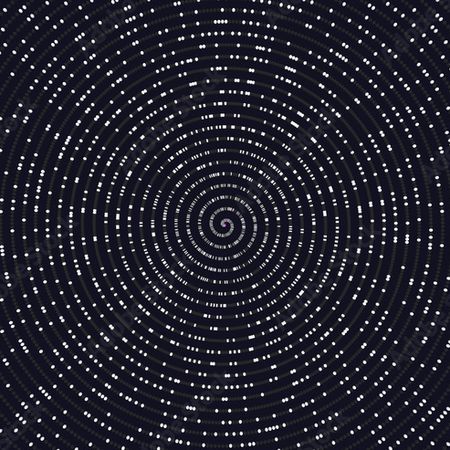
Figure 6 is a graph of all 525 input values in the complex plane. Again, I want to acknowledge that considering a two-dimensional grid of points as an input into a function may be difficult to grasp. But keep your mind open as we are arriving at the main event. What will be the output from the zeta function when we feed these 525 complex numbers as input? You likely don’t know the answer, but hopefully you are curious to learn. We could just crank through the numbers and show the output. Instead, let’s develop our intuition for what the output will be.

An intuition of continuity

I’m just getting you warmed up to think of the complex plane as an input, and I want you to take a moment and return to the usual one-dimensional input, where we input a real number and output a real number. If we were to graph the zeta function by only allowing real numbers as input within the range from 1.6 to 4.0, we could graph it in the usual $xy$-coordinate system. My question is: if we did that, would we expect a smooth curve as an output? Most functions we normally encounter are “smooth” unless there is some jump built into the function. The idea is if we take a small change in the input, say from 1.6 to 1.60001, then we would expect a small change in the output. We could scrutinize each term of the zeta function but, on the surface, there doesn’t seem to be any hiccups or jumps. This, of course, is based on our assumption the real numbers are greater than 1. We’re not going to prove it, but our intuition is that the zeta function is a continuous function when we only input real numbers into the function.

Now, if we make a small change in the imaginary component, do we have the same intuition? The way to think about it is what happens if our input is in the form of $1.6+xi$ where $x$ is a real number between -1 and +1. Our question is the same. If we make a small change to $x$, will we produce a small change in the output? Again, we’re not going to prove this, but we want to develop an intuition of a continuous process. That means we want to think that there are no jumps or hiccups to the output when we make a small change to the input. To build that intuition, recognize that when we make a small change to $x$, we are applying our coil concept. Remember that the imaginary component is about changing direction, not distance. Thus, if we consider the points $1.6+0\times i$ and $1.6+0.0001\times i$ both points will produce a “snake with the same length” because they share the same real number input. The output for the first number is only a real number, so the shape of the snake is perfectly straight. The second input number only has a small imaginary component so, even though there will be a “coil,” it will only be slight. The principle is the more we increase the imaginary component, the more we increase the coil. The intuition is there is a smooth continuity to the coiling process just like there is to the change in the length of the snake.

In summary, we should have confidence that there is a smoothness to the result if we hold an imaginary number constant and only change the real number because this will produce only a small change in the length of the snake. Likewise, holding a real number constant and only changing the imaginary number will produce only a small change in the coil of the snake without changing the length of the snake.

Capturing the zeta function in a big picture

Based on this intuition, let’s feed the input numbers into the zeta function and witness what comes out. We’re only interested in the big picture here, so we will not look at detailed calculations. With that said, there aren’t any new math concepts that we have not covered, so if you are curious, you can reproduce the results in a spreadsheet with a high degree of accuracy.

Let’s begin by considering the first column of input items where the real input is 1.6 and the imaginary input ranges from -1$i$ to +1$i$. First, if we ignore the imaginary component and only input the real number 1.6, the result is about 2.286. We can think of that as the length of the snake. If you want to think about this in our Euler formula, you can return to Figure 1 to see how each step moved left to right on the real number axis. For this example, the total distance traveled after the infinite number of steps is about 2.286.

Now, we coil the snake as we include an imaginary component. The largest imaginary number we’re considering is $i$. If we want to view the largest coil, feed $1.6+i$ into the zeta function and the result is $1.066-0.668i$. Likewise, if we feed $1.6-i$ into the zeta function, the result is $1.066+0.668i$. Figure 7 is the graph of the inputs and outputs for all 21 points. Notice in the process, we’re practicing viewing a two-dimensional input and a two-dimensional output. Since all these dots are based on the same real number 1.6, then the total distance traveled for each output is the same 2.286. But, because we have an imaginary component, we introduce rotation and our coil concept, so we circle around similar to what we did in Figure 2 for the Euler equation. We’re not showing the individual steps for this example but the concept is the same.

The solid dots which follow a circular pattern are the outputs, whereas the hollow circles in the straight line are the inputs with the real number equal to 1.6. I identified where the point $(1.6,i)$ maps to $(1.066,-0.668i)$ using a dashed line and where the point $(1.6,-i)$ maps to the point $(1.066,0.668i)$ using a solid line. Notice the positive imaginary input produces a negative imaginary output, and the negative imaginary input produces a positive imaginary output. Even though the input items are equally spaced in intervals 0.1$i$, observe the output items are not equally spaced. The dots on the far left are closer together than the dots on the far right. That indicates that even though the amount of coiling increases as we increase the imaginary component, the rate of coiling is decreasing as we increase our imaginary component.

Most of the input points are not connected to their corresponding output point, but the mapping connects as we would logically anticipate. For example, the input point nearest $(1.6,-i)$, which is $(1.6,-0.9i)$, maps to the output point nearest the point $(1.066,-0.668i)$. If you connect each input dot to each output dot in this manner, you would observe all the negative $i$ inputs map to positive $i$ outputs and all the positive $i$ inputs map to negative $i$ outputs. As we mentioned, when $i=0$ for the input, the output is 2.286 which remains on the horizontal axis.

Reviewing the other three sets of boundary input points

What do you think the results will be as we consider the other end of our range where the real input is 4.0? If there is no imaginary component, then the output is about 1.082, which is the “length of the snake” for all these points. Again, our inputs are part of the vertical line segment with the real number equal to 4.0. Like we saw with the real number input 1.6, the output is also a symmetrical curve. Figure 8 is the graph of the inputs and outputs when the real input is equal to 4.0. Now, all the output points are to the left of the input points and the curved output is much smaller.

Notice we shifted the input 2.4 units to the right from 1.6 to 4.0. I identified the end points of mapping $(4.0,i)$ to $(1.054,-0.058i)$ and $(4.0,-i)$ to $(1.054,0.058i)$. Do you recognize how the output compares to the previous output? Here are three things I noticed. First, the outputs are shifted farther to the left. They are now close to 1. We expect that since $s$ is a negative exponent in the zeta function. Increasing $s$ will decrease the result for each term. Second, the graph is more compact as the outputs are much closer to the horizontal axis. This is simply because, all things equal, a shorter snake will coil less. Third, the positive $i$ input is mapped to a negative $i$ output, a negative $i$ input is mapped to a positive $i$ output, and symmetry is preserved.

Now that we have reviewed the extreme inputs (1.6 and 4.0) for the real numbers, let’s do the same research by fixing the imaginary numbers and changing the real numbers. That means we will change the length of the snake while the “coil factor” remains constant. Again, we’ll consider the extreme imaginary number. First, set $i=-1.0$, the smallest value we are considering. Then, we’ll consider all real numbers from 1.6 to 4.0 in increments of 0.1 as before.

Figure 9 retains our convention of using solid dots as the output and the hollow circles as the input. We have already identified that the point $(1.6,-i)$ maps to $(1.066,0.668i)$ and the point $(4.0,-i)$ maps to $(1.054,0.058i)$. As expected, all negative $i$ inputs map to positive $i$ outputs. Also consistent with previous results, the equally spaced inputs do not produce equally spaced outputs. The dots at the lower part of the output are closer together than the dots above them. This indicates that the output dots are merging closer together as the real number input increases. As before, the input point nearest $(1.6,-i)$ maps to the output point nearest $(1.066,0.668i)$, preserving the idea of continuity.

Now that you have observed 3 out of the 4 extreme cases, what do you think will be the result of the fourth extreme case? The fourth extreme case fixes $i=1.0$ and considers the real input from 1.6 to 4.0. You should expect to see a mirror image of the previous case, and Figure 10 does not disappoint these expectations.

Because this is the mirror image, all the positive $i$ inputs (hollow circles) map to negative $i$ outputs (solid dots), and we have the same spacing and shape patterns as the previous case.

Reviewing the entire output from our domain

Very good. Now that we have reviewed the extreme cases individually, let’s review the extreme cases together. Figure 11 is the output for the input $(1.6,0i)$ and the 4 extreme cases we have reviewed so far.

You should be able to identify the input for each extreme case. Now that we’ve reviewed the extreme cases and have an intuition for a continuous process at play, we should anticipate that the output for all the points simply completes the pattern. Figure 12 is our complete picture of output for the inputs we have defined. You should be able to predict the general shape of the output as we have a smooth function that provides symmetry in multiple ways.

I maintained using a solid dot for the extreme output results. For outputs other than the extreme points, I used an “x.” Using symmetry, you should be able to identify where each output originated. I marked a few points to provide clues.

Reflection

Wasn’t that a fascinating journey into the complex plane? I mainly shared this because I found it fun and beautiful, and I don’t think we should keep fun and beautiful things to ourselves. But, upon reflection, there are other reasons I shared this example. One reason is to introduce the idea of using complex numbers as input into a function. It likely felt odd to use complex numbers as input. But with practice, it can feel as natural as inputting only real numbers. A second reason for sharing this is to develop an intuition for working in the complex plane of input and output and to see the symmetry and continuity of the output. Of course, we just reviewed a small sample of this function. We could review the result for any complex number input where the real number is greater than 1.

But the story of the Riemann zeta function is not limited to this domain. In fact, it is barely the beginning. That leads to another reason I shared this example. Once we move from using real number inputs to complex number inputs, we opened the door to possibilities that did not exist before. It is a classic example of the wonder and surprise that awaits us when we explore new ideas in math. There is an incredible amount of research that has been made to understand this function better. You may wonder why this simple function has created so much attention. Riemann certainly created new math real estate by using complex numbers as input. But our journey so far has only focused on the real estate that is east of the line where $s=1$. In order to understand the real pioneer work for Riemann, we must travel west, to the wild west of the line where $s<1$. The Riemann zeta function became world famous when Mr. Riemann extended the valid input values for real numbers less than 1.

More creative math

If we input $s=1$ into the zeta function, we already identified the result trails off to infinity and cannot be captured by a finite complex plane. We’ve also identified the principle that as we increase the real number input, the length of the snake gets smaller. That means we can also say the length of the snake gets larger as we decrease the real number input. Since the real number 1 produces an infinite result, what hope do we have for going further west of $s=1$ to identify anything that is meaningful? We could sample a few terms of the zeta function and quickly realize that every term is larger when $s=0.5$, for example, compared to when $s=1$. Thus, by going further west, it doesn’t appear that there is any land that we can use in our finite exploration.

This is true if we follow the rules. But the results for the zeta function are so beautiful for $s>1$. Wouldn’t it be nice if we could “imagine” results for $s<1$? This math drama should be a familiar story. Recall what we did when we could not find a solution to the equation $x^2=-1$. Our creative solution there was to define an imaginary number and run with it. Well, we’ve been “running with it” in this story, and it has been fascinating. Remember we do not like to break rules in math. However, we are perfectly fine with creating new rules as long as we preserve basic principles already in place. What is our new “rule”?

Our new “rule” is a special technique called analytic continuation. In short, using analytic continuation allows us to input complex numbers for real numbers less than 1. Rather than just plugging numbers into the formula and chugging numbers out, analytic continuation uses rule-based criteria that determine how the input numbers convert to output numbers. The specific rules for analytic continuation are complicated and beyond the scope of Lazarus Math.

The key concept for us is that the rules of analytic continuation results in a single definition for the output. That means that using analytic continuation yields one and only one output for each input in this extended domain. In other words, based on the result of the function where it is defined, which is any real number greater than 1, and based on the rules of analytic continuation, we can identify exactly one output in the complex plane for each input where the real number is less than 1.

We saw this concept at play when we defined $i=\sqrt{-1}$. Once we made that definition, then there was only one answer when we squared $i$. Thus, we used existing rules to identify the single result for $i^2=-1$. We could square both sides again and identify a single result for $i$ raised to the 4th power: $i^4=1$.

In short, we extend the domain to west of $s=1$ by using a new technique called analytic continuation. Then, we must follow the rules for analytic continuation to identify what the new graph is west of $s=1$.

Rules to the creative process

It is not a question about whether it is right or wrong to extend the domain. Rather, it is a question of remaining consistent with the principles. We move forward with the math based on the assumptions that we made to extend the math. That creates an opportunity for pioneering work to discover the results of this new math. Then, if we want to know the result of the zeta function when $s = \frac{1}{2}$, we need to know whether the function has been extended through analytic continuation. We will learn more about how we use analytic continuation to extend the zeta function in the next section. We will also learn one more interesting story about Riemann that adds to his amazing career.

Being a math artist

We often think of doing math as calculating. If we have this perspective, in a sense, we are just glorified calculators. After reviewing Riemann’s work and creating interesting and beautiful output on a two-dimensional plane, I get the feel of Riemann as also an artist who is painting a picture. His “tools” are the complex numbers and the zeta function. His canvas is the output on the complex plane.

Do you consider your math as a form of art? I believe you have a beautiful math picture already inside of you ready to be created.